Specifying Surface Aerosol Emissions for Simulations with Multi-Modal Aerosol#
Here we provide an approach to attribute size-resolved aerosol surface fluxes with individual aerosol modes used in LES and SCM
Surface fluxes are taken from Jaegle et al. (2011) and aerosol modes determined from ground-based in-situ observations
Aerosol modes help to obtain an aerosol diameter to split surface fluxes into two groups.
Below approach delivers the fraction of total number flux (i.e., intergrated over all sizes) attributed to each of two modes
While the total flux may change (e.g., from windspeed), the fraction remains constant.
import pandas as pd
import numpy as np
import matplotlib.pyplot as plt
## use coefficients by Jaegle et al. (2011) to generate a small data base of surface flux size distribution
SST = 5
vh = 20
STEP = 0.001
JAEGLE_DAT = pd.DataFrame()
## loop over a range of diameters
for DD in np.arange(0.01,8.,STEP):
A = 4.7*(1 + 30 * (DD/2))**(-0.017*(DD/2)**(-1.44))
B =(0.433 - np.log(DD/2))/0.433
SST_TERM = (0.3 + 0.1*SST - 0.0076*SST**2.0 + 0.00021*SST**3.0)
FN = SST_TERM*1.373*vh**3.41*(DD/2)**(-A)*(1+0.057*(DD/2)**3.45)*10**(1.607*np.exp(-B**2.0)) / 100 /100
## store in data frame
TMP = pd.DataFrame([[DD/2,FN,vh,SST]],columns=['Dp','FN','vh','SST'])
JAEGLE_DAT = pd.concat([JAEGLE_DAT,TMP])
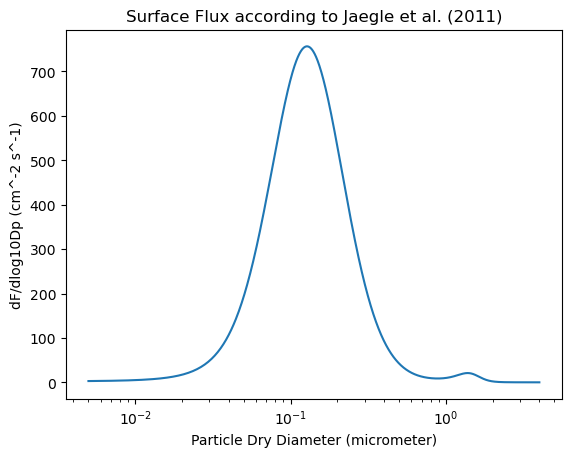
plt.plot(JAEGLE_DAT['Dp'],JAEGLE_DAT['FN'])
plt.xscale("log",base=10)
plt.xlabel('Particle Dry Diameter (micrometer)')
plt.ylabel('dF/dlog10Dp (cm^-2 s^-1)')
plt.title('Surface Flux according to Jaegle et al. (2011)')
Text(0.5, 1.0, 'Surface Flux according to Jaegle et al. (2011)')
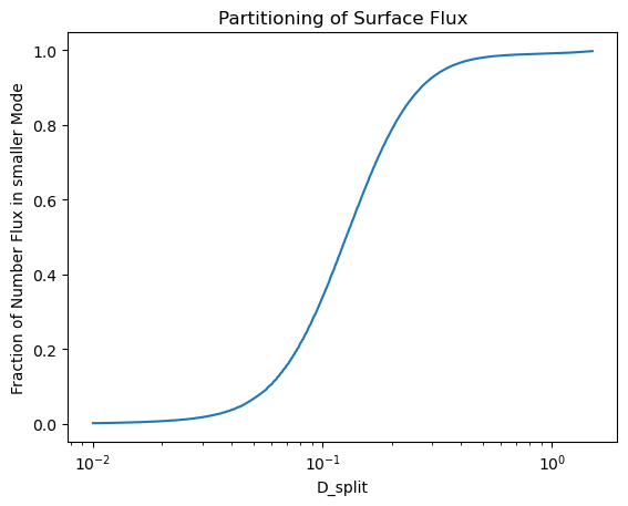
## partition into two groups and integrate over size
def split_flux(DAT,D_s,STEP):
    num_1 = np.sum(DAT.loc[DAT['Dp'] <  D_s - STEP/2]['FN'] * np.log10((DAT.loc[DAT['Dp'] <  D_s - STEP/2]['Dp']+STEP) / DAT.loc[DAT['Dp'] <  D_s- STEP/2]['Dp']))
    num_2 = np.sum(DAT.loc[DAT['Dp'] >= D_s - STEP/2]['FN'] * np.log10((DAT.loc[DAT['Dp'] >= D_s - STEP/2]['Dp']+STEP) / DAT.loc[DAT['Dp'] >= D_s - STEP/2]['Dp']))

    return [num_1/(num_1 + num_2),num_2/(num_1 + num_2)]

PARTITION_DAT = pd.DataFrame()
## loop over a range of diameters
for DD_split in np.arange(np.log(0.01),np.log(1.5),0.01):
    TMP = split_flux(JAEGLE_DAT,D_s = np.exp(DD_split),STEP=STEP)
    TMP_DAT = pd.DataFrame([[TMP[0],TMP[1],np.exp(DD_split)]],columns=['num_1','num_2','D_split'])
    PARTITION_DAT = pd.concat([PARTITION_DAT,TMP_DAT])
plt.plot(PARTITION_DAT['D_split'],PARTITION_DAT['num_1'])
plt.xscale("log")
plt.xlabel('D_split')
plt.ylabel('Fraction of Number Flux in smaller Mode')
plt.title('Partitioning of Surface Flux')
Text(0.5, 1.0, 'Partitioning of Surface Flux')
## utilize modes as specified by aerosol team (i.e., A. Williams and L. Russell)
PSD_zsm = pd.read_excel('https://docs.google.com/spreadsheets/d/' +
'1q4YkJc5dF-ZOIx-xWU_IkmTYCUPoM0kODj5ro_7Vg_c' +
'/export?gid=0&format=xlsx',
sheet_name='PSD')
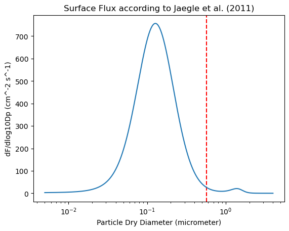
## apply simple determination of splitting point based on middle mode
D_split = np.exp(np.log(PSD_zsm['D_g'][1]*1000) + 3*np.log(PSD_zsm['sigma_g'][1]))/1000
print('Splitting modes at ' + str(D_split) + 'um')
## look up proportion of flux
PARTITION_DAT['Dp_dist'] = np.abs(PARTITION_DAT['D_split'] - D_split)
PARTITION_DAT.loc[PARTITION_DAT['Dp_dist']==PARTITION_DAT['Dp_dist'].min()]
Splitting modes at 0.5734399999999995um
| num_1 | num_2 | D_split | Dp_dist | |
|---|---|---|---|---|
| 0 | 0.98454 | 0.01546 | 0.573975 | 0.000535 |
#plt.plot(PARTITION_DAT['D_split'],PARTITION_DAT['num_1'])
plt.axvline(x = D_split, color = 'r', ls='dashed',label = 'Splitting point determined from prevalent aerosol modes')
#plt.xscale("log")
#plt.xlabel('D_split')
#plt.ylabel('Fraction of Number Flux in smaller Mode')
#plt.title('Partitioning of Surface Flux')

plt.plot(JAEGLE_DAT['Dp'],JAEGLE_DAT['FN'])
plt.xscale("log",base=10)
plt.xlabel('Particle Dry Diameter (micrometer)')
plt.ylabel('dF/dlog10Dp (cm^-2 s^-1)')
plt.title('Surface Flux according to Jaegle et al. (2011)')
Text(0.5, 1.0, 'Surface Flux according to Jaegle et al. (2011)')
Jaegle et al. (2011) surface particle flux integrated over all sizes#
\(\text{SST}\) is sea surface skin temperature in °C
\(v_h\) is horizontal wind speed at 10 m
\(F_N\) in particle number per square centimeter and second
For example, fluxed into the lowest atmospheric layer: \(S_{srf} = \frac{F_N 10^4}{\rho \Delta z}\)