Aerosol specification#
Contributed by Abigail Williams and Lynn Russell
Overview#
The aerosol specification is a parameterized particle size distribution (PSD) made up of three lognormal modes:
Mode 1 |
Mode 2 |
Mode 3 |
|
|---|---|---|---|
Na (mg-1) |
45.7 |
105.5 |
1.6 |
Dg (\(\mu\)m) |
0.04 |
0.14 |
0.50 |
\(\sigma\)g |
1.7 |
1.6 |
1.7 |
Kappa |
0.3 |
0.5 |
0.9 |
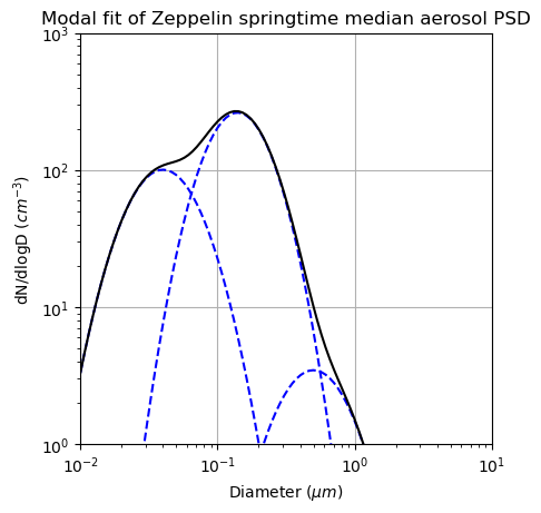
The above values are modal fits to the median aerosol PSD measured at Zeppelin Observatory in Svalbard (~1000 km upwind of COMBLE) during March-May 2020. We refer to this size distribution as PSDZSM where ZSM stands for Zeppelin-Observatory Springtime Median. Kappa values are informed by the analysis of filter measurements of aerosol composition at Zeppelin Observatory and HTDMA measurements during COMBLE.
Let’s plot PSDZSM below.
Imports#
import pandas as pd
import numpy as np
import matplotlib.pyplot as plt
Read data from Google Sheets#
The PSDZSM parameters are stored in a google sheet here. Let’s read in that data.
PSD_zsm = pd.read_excel('https://docs.google.com/spreadsheets/d/' +
                        '1q4YkJc5dF-ZOIx-xWU_IkmTYCUPoM0kODj5ro_7Vg_c' +
                        '/export?gid=0&format=xlsx',
                        sheet_name='PSD')
PSD_zsm.rename(columns={'D_g':'D_g (um)'},inplace=True)
PSD_zsm.rename(columns={'N_a':'N_a (cm^-3)'},inplace=True)
PSD_zsm.insert(2,'N_a (mg^-1)',np.round(PSD_zsm['N_a (cm^-3)']/1.27,1))
PSD_zsm
| Mode | N_a (cm^-3) | N_a (mg^-1) | D_g (um) | sigma_g | kappa | |
|---|---|---|---|---|---|---|
| 0 | Aitken | 58 | 45.7 | 0.04 | 1.7 | 0.3 |
| 1 | Accumulation | 134 | 105.5 | 0.14 | 1.6 | 0.5 |
| 2 | Sea Spray | 2 | 1.6 | 0.50 | 1.7 | 0.9 |
Calculate the size distribution#
The lognormal distribution described by the above modal parameters is defined by the equation below (following Seinfeld and Pandis 2016):
Let’s calculate the size distribution corresponding to the PSDZSM parameters.
#create a diameter array
D = np.logspace(-2, 1, num=100)

#calculate lognormal mode number size distribution
PSD_mode1 = np.multiply(np.divide(PSD_zsm.at[0, 'N_a (cm^-3)'], (np.sqrt(2 * np.pi) * np.log10(PSD_zsm.at[0, 'sigma_g']))), \
                        np.exp(-(np.square(np.subtract(np.log10(D), np.log10(PSD_zsm.at[0, 'D_g (um)'])))) \
                               / (2 * np.square(np.log10(PSD_zsm.at[0, 'sigma_g'])))))
PSD_mode2 = np.multiply(np.divide(PSD_zsm.at[1, 'N_a (cm^-3)'], (np.sqrt(2 * np.pi) * np.log10(PSD_zsm.at[1, 'sigma_g']))), \
                        np.exp(-(np.square(np.subtract(np.log10(D), np.log10(PSD_zsm.at[1, 'D_g (um)'])))) / \
                               (2 * np.square(np.log10(PSD_zsm.at[1, 'sigma_g'])))))
PSD_mode3 = np.multiply(np.divide(PSD_zsm.at[2, 'N_a (cm^-3)'], (np.sqrt(2 * np.pi) * np.log10(PSD_zsm.at[2, 'sigma_g']))), \
                        np.exp(-(np.square(np.subtract(np.log10(D), np.log10(PSD_zsm.at[2, 'D_g (um)'])))) / \
                               (2 * np.square(np.log10(PSD_zsm.at[2, 'sigma_g'])))))

#sum three individual lognormal modes together to make a single tri-modal size distribution
PSD_sum = PSD_mode1 + PSD_mode2 + PSD_mode3
Plot the PSD#
plt.plot(D, PSD_mode1, '--b')
plt.plot(D, PSD_mode2, '--b')
plt.plot(D, PSD_mode3, '--b')
plt.plot(D, PSD_sum, 'k')
plt.axis('square')
plt.yscale('log')
plt.xscale('log')
plt.xlim([1e-2, 1e1])
plt.ylim([1e0, 1e3])
plt.grid()
plt.xlabel('Diameter $(\mu m)$')
plt.ylabel('dN/dlogD $(cm^{-3})$')
plt.title('Modal fit of Zeppelin springtime median aerosol PSD')
plt.show()
References#
We thank Radovan Krejci, Paul Zieger, and Peter Tunved for supplying the dataset of aerosol measurements taken at Zeppelin Observatory.
A manuscript detailing aerosol characteristics during cold-air outbreaks around the Norwegian Sea is now published (Williams et al., 2024). This manuscript further describes the observations and methods used to derive the above parameters for the modal fit to the springtime median aerosol PSD at Zeppelin Observatory.