DEPHY Forcing Derivation#
Developed by Tim Juliano (NCAR-RAL), Ann Fridlind (NASA-GISS), and Florian Tornow (NASA-GISS/Columbia Univ.) with substantial contributions by Peng Wu (PNNL), Gunilla Svensson (Stockholm Univ.), and Andy Ackerman (NASA-GISS)
v2.4 created on 1/24/24
Thanks to Jan Chylik (University of Cologne) for pointing out fix to global attributes
Based on ERA5 backward trajectory, beginning at Andenes, Norway (03/13/20 at 18 UTC)
We have the option of starting as far as 28 hours before arriving at Andenes (03/12/20 at 14 UTC)
Import libraries#
import numpy as np
import numpy.ma as ma
import sys
from netCDF4 import Dataset, date2num
import datetime as dt
import os
import matplotlib.pyplot as plt
from scipy import interpolate
import geopy.distance
from scipy.ndimage import gaussian_filter1d
User mods#
How many hours before ice edge do you want to start?
Note: Value == 0 means you are starting approx. at ice edge, Value == 10 means you are starting 10 h upstream (north) of the ice edge
Note: Value must be an integer
Note: t0_h represents simulation start time, t0_h_init_th_qv represents initial theta/qv profile to use; set equivalent if everything should be initialized using information at same time
t0_h = 2
t0_h_init_th_qv = 5
if t0_h < 0 or t0_h > 10:
    sys.exit('Error: Please set 0 <= t0_h >= 10')
Clobber old forcing file?
clobber_old_file = True
Forcing file save name
Note: For this and all file paths, include directory in the name
save_name = 'COMBLE_INTERCOMPARISON_FORCING_V2.4.nc'
Name of current script for global attribute
Note: Can use ipynbname library to automatically generate script name, but this is not a standard library so skipping for now
script_name = 'create_comble_forcing_v2.4.ipynb'
LES domain locations
fname_les_domain = 'LES_domain_location_28h_18Z_Mar13_2020.txt'
ERA5 backward trajectory met file name
fname_era5_met = 'theta_temp_rh_sh_uvw_sst_along_trajectory_era5ml_28h_end_2020-03-13-18_v2.nc'
ERA5 backward trajectory ozone file name
fname_era5_o3 = 'ERA5_forcing_along_trajectory_end_2020-03-13-18.nc'
1D model profiles file name
profiles_1d_model = 'u_v_theta_z.txt'
Sea ice concentration file name
fname_sic = 'Svalbard_asi-AMSR2-n10m-20200313_m.nc'
Do geostrophic wind calc and add to forcing file? If so, supply ERA5 geopotential height file name and minimum grid spacing (km) for discretization
do_geo = True
if do_geo:
    fname_era5_geo = '/glade/derecho/scratch/tjuliano/doe_comble/wrf_asr_cao/WRF-ASR-CAO/scripts/era5/era5_mar13_case_larger.nc'
    min_dx = 20.
    min_dy = 20.
Add theta and qv nudging, as well as subsidence, to forcing file?
do_u_v_nudge = True
do_th_qv_nudge = True
do_subsidence = True
Set things for future calculations#
Note: no need for user to modify these, computed automatically
Timings
nhrs = 18 + t0_h + 1 # total number of simulation hours, including t0
if t0_h == 0:
    start_time = '2020-03-13 00:00:00'
    start_day = 13
    start_hour = 0
else:
    start_time = '2020-03-12 ' + str(24-t0_h) + ':00:00'
    start_day = 12
    start_hour = 24-t0_h
print ('Start time is: ' + start_time)
Start time is: 2020-03-12 22:00:00
Constants for geostrophic wind calc
if do_geo:
    omega = 7.2921e-5 # angular velocity
    g = 9.81 # grav constant
Delete forcing file if already exists
if clobber_old_file:
    if os.path.exists(save_name):
        os.remove(save_name)
        print('The file ' + save_name + ' has been deleted successfully')
The file COMBLE_INTERCOMPARISON_FORCING_V2.4.nc has been deleted successfully
Get LES domain locations
les_loc = np.loadtxt(fname_les_domain,skiprows=1)
les_hh = les_loc[:,0]
les_hh_idx = np.where(les_hh>=-1.*t0_h)[0]
les_lat = les_loc[les_hh_idx,1]
les_lat2 = les_lat[::12]
les_lon = les_loc[les_hh_idx,2]
les_lon2 = les_lon[::12]

les_lat_mid = round(np.mean(les_lat),1)
les_lon_mid = round(np.mean(les_lon),1)
print ('LES domain mid point: ' + 'lat=' + str(les_lat_mid) + 'N, lon=' + str(les_lon_mid) + 'E')
LES domain mid point: lat=74.5N, lon=9.9E
Create vertical grid#
160 vertical grid levels, defined at the cell faces
nz = 160

dz_grid = np.empty(nz-1)
dz_grid[0] = 20.0
dz_grid[1] = 25.0
dz_grid[2] = 30.0
dz_grid[3] = 35.0
dz_grid[4:140] = 40.0
dz_grid[140] = 60.0
dz_grid[141:157] = 80.0
dz_grid[157] = 60.0
dz_grid[158] = 50.0

z_grid = np.empty(nz)
z_grid[0] = 0.0
for i in np.arange(1,len(z_grid)):
    z_grid[i] = z_grid[i-1] + dz_grid[i-1]
Read in data from ERA5 backtrajectory (netCDF)#
# Open met dataset
dataset = Dataset(fname_era5_met, "r")

# Read variables (1D arrays are time, 2D arrays are time x pressure level)
hours = dataset.variables['Time'][:]
lat = dataset.variables['Latitude'][:]
lon = dataset.variables['Longitude'][:]
pres = dataset.variables['Pressure'][:,:]
sfc_pres = dataset.variables['SfcPres'][:]
sst = dataset.variables['SST'][:]
hgt = dataset.variables['GEOS_HT'][:,:]
uwnd = dataset.variables['U'][:,:]
vwnd = dataset.variables['V'][:,:]
wwnd = dataset.variables['W'][:,:]
temp = dataset.variables['Temp'][:,:]
theta = dataset.variables['Theta'][:,:]
qv = dataset.variables['SH'][:,:]

# Open ozone dataset
dataset_o3 = Dataset(fname_era5_o3, "r")

# Read variables
o3 = dataset_o3.variables['O3'][:,:]
pres_o3 = dataset_o3.variables['Pressure'][:]
Convert units
pres_pa = pres*100.          # hPa to Pa
pres_o3_pa = pres_o3*100.    # hPa to Pa
Reverse time dimension of 2D arrays, as well as sfc pressure and sst, so that beginning of backward trajectory is in first position
hgt = np.flip(hgt,axis=0)
uwnd = np.flip(uwnd,axis=0)
vwnd = np.flip(vwnd,axis=0)
wwnd = np.flip(wwnd,axis=0)
temp = np.flip(temp,axis=0)
theta = np.flip(theta,axis=0)
pres_pa = np.flip(pres_pa,axis=0)
qv = np.flip(qv,axis=0)
o3 = np.flip(o3,axis=0)
sfc_pres = sfc_pres[::-1]
sst = sst[::-1]
Unmask sst field and get index according to t0_h (furthest north we can go is 28h after backtrajectory initialization from Andenes, or 3/12/20 at 14 UTC)
sst_real = ma.getdata(sst)
loopidx = np.where(sst_real>0.0)[0]
t0 = loopidx[10-t0_h]
t0_init_th_qv = loopidx[10-t0_h_init_th_qv]
Calculate sfc potential temperature
theta1000mb = theta[:,0]
sfc_theta = theta1000mb*pow((100000./sfc_pres),0.286)
Get information at t0
z1 = 0

pres_t0 = pres_pa[t0,z1:]
pres_o3_t0 = pres_o3_pa[z1:]
hgt_t0 = hgt[t0_init_th_qv,z1:]
uwnd_t0 = uwnd[t0,z1:]
vwnd_t0 = vwnd[t0,z1:]
wwnd_t0 = wwnd[t0,z1:]
temp_t0 = temp[t0_init_th_qv,z1:]
theta_t0 = theta[t0_init_th_qv,z1:]
qv_t0 = qv[t0_init_th_qv,z1:]

# temporal avg for o3
o3_t0 = np.mean(o3[0:18+t0_h+1,z1:],axis=0)

ps_t0 = sfc_pres[t0]
thetas_t0 = sfc_theta[t0]
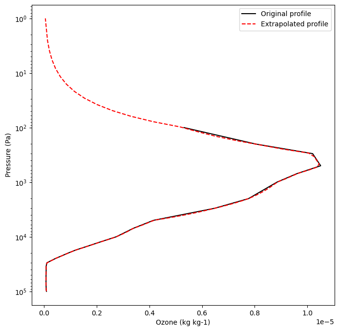
Extrapolate O3 since ERA5 only goes to 1 hPa and plot versus original profile
# Add top pressure and o3 value - here we assume o3 goes to zero at 1e-4 Pa
pres_o3_t0_add_top = np.insert(pres_o3_t0,len(pres_o3_t0),0.0001)
o3_t0_add_top = np.insert(o3_t0,len(o3_t0),0.0)

# Add bottom pressure and o3 value - here we assume o3 is constant near the sfc
pres_o3_t0_add_top_bottom = np.insert(pres_o3_t0_add_top,0,pres_t0[0])
o3_t0_add_top_bottom = np.insert(o3_t0_add_top,0,o3_t0[0])

# Do the extrapolation
f = interpolate.interp1d(pres_o3_t0_add_top_bottom, o3_t0_add_top_bottom, kind='linear',fill_value='extrapolate')
o3_t0i = f(pres_t0.data)

plt.figure()
plt.figure(figsize=(8,8))

var_plt1 = o3_t0
var_plt2 = o3_t0i
plt.plot(var_plt1,pres_o3_t0,c='k',label='Original profile')
plt.plot(var_plt2,pres_t0,c='r',ls='--',label='Extrapolated profile')
plt.legend()
plt.xlabel('Ozone (kg kg-1)')
plt.ylabel('Pressure (Pa)')
plt.yscale('log')
plt.gca().invert_yaxis()

plt.show()
<Figure size 640x480 with 0 Axes>
Get Geostrophic wind forcing#
if do_geo:
    # Read ERA5 file
    dataset = Dataset(fname_era5_geo, "r")

    zl = dataset.variables['z'][24-t0_h:43,0:-1,:,:] # time, lev, lat, lon
    lonarrl = dataset.variables['longitude'][:]
    latarrl = dataset.variables['latitude'][:]

    latloc = np.empty(len(les_lat2),dtype=np.int16)
    lonloc = np.empty(len(les_lat2),dtype=np.int16)
    ugl = np.empty([len(les_lat2),np.shape(zl)[1]])
    vgl = np.empty([len(les_lat2),np.shape(zl)[1]])
    zhtl = np.empty([len(les_lat2),np.shape(zl)[1]])

    for i in np.arange(len(les_lat2)):
        hold = np.abs(les_lat2[i]-latarrl)
        latloc[i] = np.argmin(hold)
        hold = np.abs(les_lon2[i]-lonarrl)
        lonloc[i] = np.argmin(hold)

        # Coriolis parameter
        e = 2*omega*np.cos(np.radians(les_lat2[i]))
        f = 2*omega*np.sin(np.radians(les_lat2[i]))

        # Calc dx, dy
        offset1 = 1
        offset2 = 1
        coords_1 = (latarrl[latloc[i]], lonarrl[lonloc[i]-offset2])
        coords_2 = (latarrl[latloc[i]], lonarrl[lonloc[i]+offset2])
        dx = geopy.distance.geodesic(coords_1, coords_2).km
        coords_3 = (latarrl[latloc[i]-offset1], lonarrl[lonloc[i]])
        coords_4 = (latarrl[latloc[i]+offset1], lonarrl[lonloc[i]])
        dy = geopy.distance.geodesic(coords_3, coords_4).km
        while dx < min_dx: # we want at least min_dx km for our zonal discretization, which changes with time (latitude)
            offset2+=1
            coords_1 = (latarrl[latloc[i]], lonarrl[lonloc[i]-offset2])
            coords_2 = (latarrl[latloc[i]], lonarrl[lonloc[i]+offset2])
            dx = geopy.distance.geodesic(coords_1, coords_2).km
        while dy < min_dy: # we want at least min_dy km for our meridional discretization, which stays mostly constant with time (latitude)
            offset1+=1
            coords_3 = (latarrl[latloc[i]-offset1], lonarrl[lonloc[i]])
            coords_4 = (latarrl[latloc[i]+offset1], lonarrl[lonloc[i]])
            dy = geopy.distance.geodesic(coords_3, coords_4).km

        dx = dx*1000. # km to m
        dy = dy*1000.

        # Calc Vg
        ugl[i,:] = (-1./f) * (zl[i,:,latloc[i]-offset1,lonloc[i]]-zl[i,:,latloc[i]+offset1,lonloc[i]])/dy
        vgl[i,:] = (1/f)  * (zl[i,:,latloc[i],lonloc[i]+offset2]-zl[i,:,latloc[i],lonloc[i]-offset2])/dx
        zhtl[i,:] = zl[i,:,latloc[i],lonloc[i]]/g

    ugeo = np.flip(ugl,1)
    vgeo = np.flip(vgl,1)
    zgeo = np.flip(zhtl,1)

    ugeo = gaussian_filter1d(ugeo, 1)
    vgeo = gaussian_filter1d(vgeo, 1)

    print ('Geostrophic wind computed')
---------------------------------------------------------------------------
FileNotFoundError                         Traceback (most recent call last)
Cell In[25], line 3
      1 if do_geo:
      2     # Read ERA5 file
----> 3     dataset = Dataset(fname_era5_geo, "r")
      5     zl = dataset.variables['z'][24-t0_h:43,0:-1,:,:] # time, lev, lat, lon
      6     lonarrl = dataset.variables['longitude'][:]

File src/netCDF4/_netCDF4.pyx:2449, in netCDF4._netCDF4.Dataset.__init__()

File src/netCDF4/_netCDF4.pyx:2012, in netCDF4._netCDF4._ensure_nc_success()

FileNotFoundError: [Errno 2] No such file or directory: '/glade/derecho/scratch/tjuliano/doe_comble/wrf_asr_cao/WRF-ASR-CAO/scripts/era5/era5_mar13_case_larger.nc'
Interpolate profiles#
Interpolate/extrapolate Ug/Vg to native ERA5 levels
if do_geo:
    ugeo_new = np.empty([np.shape(ugeo)[0],np.shape(hgt)[1]])
    vgeo_new = np.empty([np.shape(ugeo)[0],np.shape(hgt)[1]])
    zgeo_new = np.empty([np.shape(ugeo)[0],np.shape(hgt)[1]])
    for i in np.arange(len(les_lat2)):
        zgeo_new[i,:] = hgt[t0+i,z1:]

        f = interpolate.interp1d(zgeo[i,:], ugeo[i,:], bounds_error=False, fill_value='extrapolate')
        ugeo_new[i,:] = f(zgeo_new[i,:].data)

        f = interpolate.interp1d(zgeo[i,:], vgeo[i,:], bounds_error=False, fill_value='extrapolate')
        vgeo_new[i,:] = f(zgeo_new[i,:].data)
Interpolate t0 profiles, nudging profiles, and geostrophic wind profiles to common vertical grid for simplicity
Find time with highest first level and get vertical grid
if do_geo:
    zz1_geo = np.empty([nhrs,len(pres_t0)])
    count = 0
    for i in np.arange(nhrs):
        zz1_geo[count,:] = zgeo_new[i,0]

        count+=1

    zz1_nudge = np.empty([nhrs,len(pres_t0)])
    count = 0
    for i in np.arange(nhrs):
        zz1_nudge[count,:] = hgt[t0+i,z1:]

        count+=1

    zz1_geo_max_idx = np.argmax(zz1_geo[:,0])
    zz1_nudge_max_idx = np.argmax(zz1_nudge[:,0])
    zz1_geo_max = zz1_geo[zz1_geo_max_idx,0]
    zz1_nudge_max = zz1_nudge[zz1_nudge_max_idx,0]

    if zz1_geo_max > zz1_nudge_max:
        zgeoi = zz1_geo[zz1_geo_max_idx,0:-1]
    else:
        zgeoi = zz1_nudge[zz1_nudge_max_idx,0:-1]

else:
    zz1_nudge = np.empty([nhrs,len(pres_t0)])
    count = 0
    for i in np.arange(nhrs):
        zz1_nudge[count,:] = hgt[t0+i,z1:]

        count+=1

    zz1_nudge_max_idx = np.argmax(zz1_nudge[:,0])
    zz1_nudge_max = zz1_nudge[zz1_nudge_max_idx,0]

    zgeoi = zz1_nudge[zz1_nudge_max_idx,0:-1]

print ('First level for all profiles = ' + str(round(zgeoi[0],3)) + ' m' )
print (zgeoi)
First level for all profiles = 18.168 m
[1.81678200e+01 3.78291588e+01 5.93531876e+01 8.29409561e+01
 1.08634644e+02 1.36762817e+02 1.67474060e+02 2.01006256e+02
 2.37572968e+02 2.77470947e+02 3.20925720e+02 3.68243713e+02
 4.19705322e+02 4.75707489e+02 5.36504822e+02 6.02413635e+02
 6.73863464e+02 7.51188721e+02 8.34781677e+02 9.25015015e+02
 1.02229761e+03 1.12704102e+03 1.23956067e+03 1.36028394e+03
 1.48945679e+03 1.62738745e+03 1.77428064e+03 1.93038416e+03
 2.09574048e+03 2.27039331e+03 2.45438965e+03 2.64754395e+03
 2.84974072e+03 3.06066577e+03 3.27992432e+03 3.50704077e+03
 3.74134668e+03 3.98210889e+03 4.22867920e+03 4.48078857e+03
 4.73797949e+03 4.99874365e+03 5.26092578e+03 5.52306201e+03
 5.78483252e+03 6.04644922e+03 6.30803760e+03 6.56951123e+03
 6.83091602e+03 7.09283643e+03 7.35596924e+03 7.62092139e+03
 7.88798877e+03 8.15741553e+03 8.42925000e+03 8.70381738e+03
 8.98155176e+03 9.26270898e+03 9.54723730e+03 9.83502930e+03
 1.01259678e+04 1.04200625e+04 1.07173477e+04 1.10177529e+04
 1.13212578e+04 1.16278047e+04 1.19373662e+04 1.22498711e+04
 1.25653350e+04 1.28839326e+04 1.32058555e+04 1.35312275e+04
 1.38601523e+04 1.41925664e+04 1.45284150e+04 1.48675010e+04
 1.52095967e+04 1.55542930e+04 1.59013115e+04 1.62505469e+04
 1.66022949e+04 1.69575215e+04 1.73173887e+04 1.76829043e+04
 1.80547246e+04 1.84334707e+04 1.88199785e+04 1.92153418e+04
 1.96205273e+04 2.00361152e+04 2.04623945e+04 2.09000508e+04
 2.13498691e+04 2.18124043e+04 2.22871719e+04 2.27734141e+04
 2.32704062e+04 2.37781934e+04 2.42975605e+04 2.48301953e+04
 2.53780762e+04 2.59425137e+04 2.65239766e+04 2.71227988e+04
 2.77392344e+04 2.83741738e+04 2.90299805e+04 2.97107168e+04
 3.04193066e+04 3.11562773e+04 3.19218848e+04 3.27171895e+04
 3.35436523e+04 3.44022461e+04 3.52931797e+04 3.62169961e+04
 3.71792188e+04 3.82055078e+04 3.93279570e+04 4.05411719e+04
 4.18197422e+04 4.31656016e+04 4.45927344e+04 4.61026953e+04
 4.76934102e+04 4.93620195e+04 5.11093516e+04 5.29429336e+04
 5.48647773e+04 5.68720195e+04 5.89728828e+04 6.11852734e+04
 6.35144883e+04 6.59572734e+04 6.85121250e+04 7.11708984e+04]
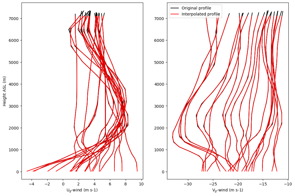
Do the linear interpolation of time-varying geostrophic profiles to new vertical grid
if do_geo:
    ugeoi = np.empty([nhrs,len(pres_t0)-1])
    vgeoi = np.empty([nhrs,len(pres_t0)-1])
    count = 0
    for i in np.arange(nhrs):
        f = interpolate.interp1d(zgeo_new[i,:], ugeo_new[i,:])
        ugeoi[count,:] = f(zgeoi)
        f = interpolate.interp1d(zgeo_new[i,:], vgeo_new[i,:])
        vgeoi[count,:] = f(zgeoi)

        count+=1
Compare original and interpolated profiles of time-varying geostrophic wind as example to show efficacy of method
zplt1 = 0
zplt2 = nhrs-3
zplt2b = 50

if do_geo:
    plt.figure()
    plt.figure(figsize=(12,8))

    var_plt1 = ugeo
    var_plt2 = ugeoi
    plt.subplot(121)
    for i in np.arange(nhrs):
        plt.plot(var_plt1[i,zplt1:zplt2],zgeo[i,zplt1:zplt2],c='k')
        plt.plot(var_plt2[i,zplt1:zplt2b],zgeoi[zplt1:zplt2b],c='r')
    plt.xlabel('U$_{g}$-wind (m s-1)')
    plt.ylabel('Height ASL (m)')

    var_plt1 = vgeo
    var_plt2 = vgeoi
    plt.subplot(122)
    for i in np.arange(nhrs):
        if i == 0:
            plt.plot(var_plt1[i,zplt1:zplt2],zgeo[i,zplt1:zplt2],c='k',label='Original profile')
            plt.plot(var_plt2[i,zplt1:zplt2b],zgeoi[zplt1:zplt2b],c='r',label='Interpolated profile')
        else:
            plt.plot(var_plt1[i,zplt1:zplt2],zgeo[i,zplt1:zplt2],c='k')
            plt.plot(var_plt2[i,zplt1:zplt2b],zgeoi[zplt1:zplt2b],c='r')
    plt.xlabel('V$_{g}$-wind (m s-1)')
    plt.legend()
    plt.show()
<Figure size 640x480 with 0 Axes>
Do the linear interpolation for initial forcing profiles
f = interpolate.interp1d(hgt_t0, pres_t0)
pres_t0i = f(zgeoi)
f = interpolate.interp1d(hgt_t0, uwnd_t0)
uwnd_t0i = f(zgeoi)
f = interpolate.interp1d(hgt_t0, vwnd_t0)
vwnd_t0i = f(zgeoi)
f = interpolate.interp1d(zgeoi, ugeoi[0,:])
ugeoi_t0i = f(zgeoi)
f = interpolate.interp1d(zgeoi, vgeoi[0,:])
vgeoi_t0i = f(zgeoi)
f = interpolate.interp1d(hgt_t0, wwnd_t0)
wwnd_t0i = f(zgeoi)
f = interpolate.interp1d(hgt_t0, temp_t0)
temp_t0i = f(zgeoi)
f = interpolate.interp1d(hgt_t0, theta_t0)
theta_t0i = f(zgeoi)
f = interpolate.interp1d(hgt_t0, qv_t0)
qv_t0i = f(zgeoi)
f = interpolate.interp1d(hgt_t0, o3_t0i)
o3_t0i = f(zgeoi)
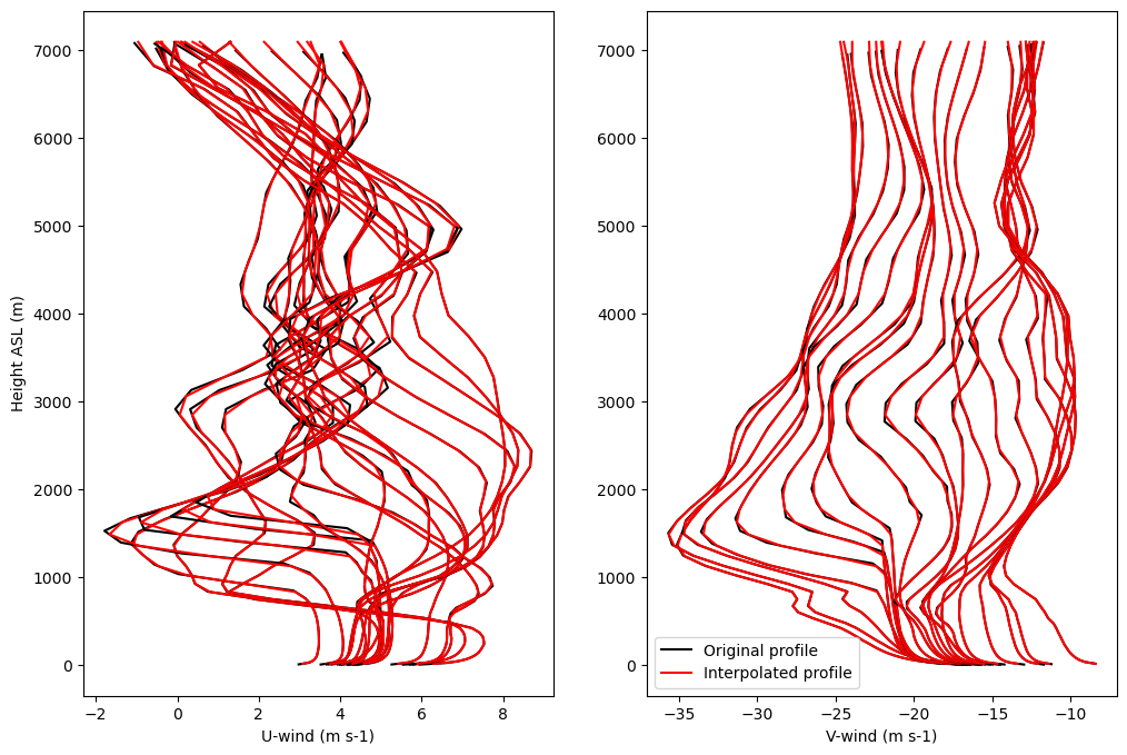
Do the linear interpolation for nudging forcing profiles
if do_u_v_nudge:
    unudgei = np.empty([nhrs,len(pres_t0)-1])
    vnudgei = np.empty([nhrs,len(pres_t0)-1])
if do_th_qv_nudge:
    tnudgei = np.empty([nhrs,len(pres_t0)-1])
    qvnudgei = np.empty([nhrs,len(pres_t0)-1])
if do_subsidence:
    wnudgei = np.empty([nhrs,len(pres_t0)-1])
count = 0
if do_u_v_nudge or do_th_qv_nudge or do_subsidence:
    for i in np.arange(nhrs):
        if do_u_v_nudge:
            f = interpolate.interp1d(hgt[t0+i,z1:], uwnd[t0+i,z1:])
            unudgei[count,:] = f(zgeoi)
            f = interpolate.interp1d(hgt[t0+i,z1:], vwnd[t0+i,z1:])
            vnudgei[count,:] = f(zgeoi)

        if do_th_qv_nudge:
            f = interpolate.interp1d(hgt[t0+i,z1:], theta[t0+i,z1:])
            tnudgei[count,:] = f(zgeoi)

            f = interpolate.interp1d(hgt[t0+i,z1:], qv[t0+i,z1:])
            qvnudgei[count,:] = f(zgeoi)
        if do_subsidence:
            f = interpolate.interp1d(hgt[t0+i,z1:], wwnd[t0+i,z1:])
            wnudgei[count,:] = f(zgeoi)

        count+=1
Compare original and interpolated profiles of time-varying nudging wind as example to show efficacy of method
zplt1 = 0
zplt2 = 50
zplt2b = 50

if do_geo and do_u_v_nudge:
    plt.figure(figsize=(12,8))

    var_plt1 = uwnd
    var_plt2 = unudgei
    plt.subplot(121)
    for i in np.arange(nhrs):
        plt.plot(var_plt1[t0+i,zplt1:zplt2],hgt[t0+i,zplt1:zplt2],c='k')
        plt.plot(var_plt2[i,zplt1:zplt2b],zgeoi[zplt1:zplt2b],c='r')
    plt.xlabel('U-wind (m s-1)')
    plt.ylabel('Height ASL (m)')

    var_plt1 = vwnd
    var_plt2 = vnudgei
    plt.subplot(122)
    for i in np.arange(nhrs):
        if i == 0:
            plt.plot(var_plt1[t0+i,zplt1:zplt2],hgt[t0+i,zplt1:zplt2],c='k',label='Original profile')
            plt.plot(var_plt2[i,zplt1:zplt2b],zgeoi[zplt1:zplt2b],c='r',label='Interpolated profile')
        else:
            plt.plot(var_plt1[t0+i,zplt1:zplt2],hgt[t0+i,zplt1:zplt2],c='k')
            plt.plot(var_plt2[i,zplt1:zplt2b],zgeoi[zplt1:zplt2b],c='r')
    plt.xlabel('V-wind (m s-1)')
    plt.legend()
    plt.show()
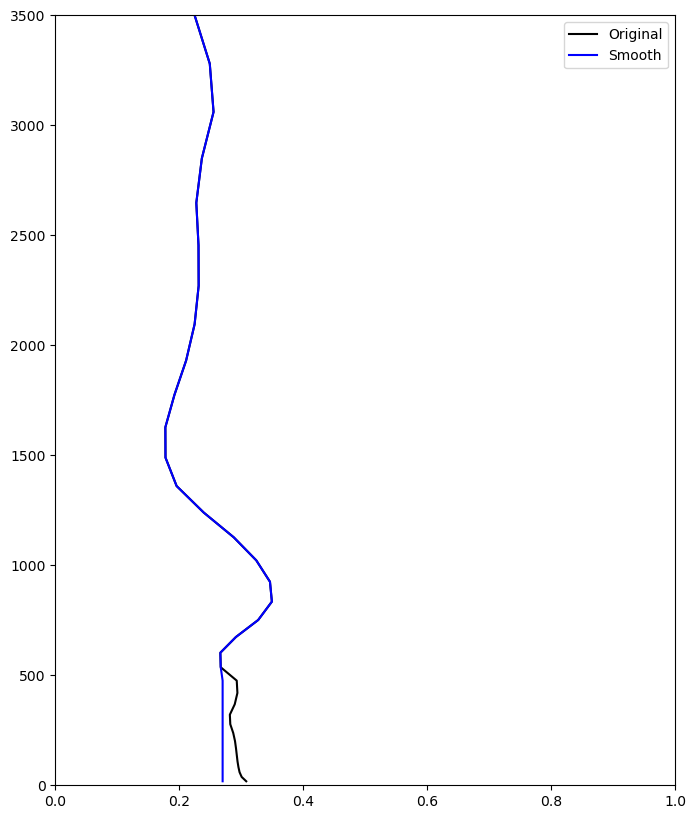
Smooth initial water vapor mixing ratio profile#
qv_t0i_mod = qv_t0i.copy()
qv_t0i_mod[0:14] = 0.27e-3

plt.figure(figsize=(8,10))
plt.plot(qv_t0i*1e3,zgeoi,c='k',label='Original')
plt.plot(qv_t0i_mod*1e3,zgeoi,c='b',label='Smooth')
plt.ylim(0,3500)
plt.xlim(0,1)
plt.legend()
<matplotlib.legend.Legend at 0x148c3c8047c0>
Do surface forcing#
Calculate sea ice concentration along trajectory
sic_file = Dataset(fname_sic)
sic = sic_file.variables['z'][:,:]
sic_lat = sic_file.variables['lat'][:]
sic_lon = sic_file.variables['lon'][:]

sic_traj = np.empty(len(les_hh_idx))
for i in np.arange(len(les_hh_idx)):
    abslat = np.abs(sic_lat-les_lat[i])
    abslon = np.abs(sic_lon-les_lon[i])
    jlat = np.argmin(abslat)
    ilon = np.argmin(abslon)
    sic_traj[i] = sic[jlat,ilon]
Get time series information for sfc forcing
# Print statements?
verbose = False

# Pack ice skin temperature
tsk_ice = 247.0

# Interpolate SST
tmp_hh = np.arange(-1*t0_h,19,1) # these are the hours we have SST data from the ERA5 backward trajectory file
f = interpolate.interp1d(tmp_hh, sst[t0:])
sst_interp = f(les_hh[les_hh_idx])

# Modification for over ice/MIZ
sst_ts = np.empty(len(sic_traj))
for i in np.arange(len(sic_traj)):
    if sic_traj[i] > 90.0: # over ice
        sst_ts[i] = tsk_ice
    elif sic_traj[i] > 0.0: # MIZ
        sst_ts[i] = (sic_traj[i]/100.)*tsk_ice + (1.-(sic_traj[i]/100.))*sst_interp[i] # MIZ
    else: # open ocean
        sst_ts[i] = sst_interp[i]
    if verbose:
        print ('Computed TSK for hour ' + str(round(5*i/60.,3)) + ': '
               + str(round(sst_ts[i],3)) + ' with SIC = ' + str(sic_traj[i]/100.) +
               ' and SST = ' + str(round(sst_interp[i],3)))

# Pull hourly SST
sst_ts = sst_ts[::12]
Create new netcdf file#
try: ncfile.close()  # just to be safe, make sure dataset is not already open.
except: pass
ncfile = Dataset(save_name,mode='w',format='NETCDF3_CLASSIC')
Create dimensions
levs = len(zgeoi)
z_grid_levs = len(z_grid)
t0_dim = ncfile.createDimension('t0', 1)     # initial time axis
lat_dim = ncfile.createDimension('lat', 1)     # latitude axis
lon_dim = ncfile.createDimension('lon', 1)     # longitude axis
lev_dim = ncfile.createDimension('lev', levs)      # level axis
zw_grid_dim = ncfile.createDimension('zw_grid', z_grid_levs)      # zw_grid axis
time_dim = ncfile.createDimension('time', None)    # unlimited axis (can be appended to)
Create global attributes
ncfile.title='Forcing and initial conditions for 13 March 2020 COMBLE intercomparison case'
ncfile.reference='https://arm-development.github.io/comble-mip/'
ncfile.authors='Timothy W. Juliano (NCAR/RAL, tjuliano@ucar.edu); Florian Tornow (NASA/GISS, ft2544@columbia.edu); Ann M. Fridlind (NASA/GISS, ann.fridlind@nasa.gov)'
ncfile.version='Created on ' + dt.date.today().strftime('%Y-%m-%d')
ncfile.format_version='DEPHY SCM format version 2.0'
ncfile.script=script_name
ncfile.startDate=start_time
ncfile.endDate='2020-03-13 18:00:00'
if do_geo:
    ncfile.forc_geo=1
else:
    ncfile.forc_geo=0
ncfile.radiation='on'
ncfile.forc_wap=0
ncfile.forc_wa=0
ncfile.nudging_u=0
ncfile.nudging_v=0
ncfile.nudging_w=0
ncfile.nudging_theta=0
ncfile.nudging_qv=0
ncfile.surface_type='ocean'
ncfile.surface_forcing_temp='ts'
ncfile.z0h='5.5e-6 m'
ncfile.surface_forcing_moisture='none'
ncfile.z0q='5.5e-6 m'
ncfile.surface_forcing_wind='z0'
ncfile.z0='9.0e-4 m'
ncfile.lat=str(les_lat_mid) + ' deg N'
ncfile.droplet_activation_diagnostic='droplet number concentration fixed to 20 cm-3'
ncfile.ice_nucleation_diagnostic='total ice number concentration fixed to 25 L-1 where qc+qr>1e-6 kg/kg and T<268.15 K'
ncfile.droplet_activation_prognostic='time and space varying aerosol initialized from na1, na2 and na3, which are uniform initial profiles to be affected by collision-coalescence processes, sea spray source, and mixing'
ncfile.aerosol_surface_source='modal emissions based on Jaegle et al. (2011)\'s size-resolved surface source fluxes (equation 4) that vary as a function of wind speed and SST; from size-integrated fluxes we determine proportional attribution to the two larger modes via modal geometric mean and standard deviation of the accumulation mode (na2); for the configuration here: 98.5% (accumulation mode, na2) and 1.5% (sea spray mode, na3)'
ncfile.ice_nucleation_prognostic='assume that all sea spray mode and half of internally mixed accumulation mode aerosols behave as ice nucleating particles in the immersion mode, and apply parameterization of choice'
Create variables
Dimensions
t0_time = ncfile.createVariable('t0', np.float32, ('t0',))
t0_time.units = 'seconds since ' + start_time
t0_time.long_name = 'Initial time'

latitude = ncfile.createVariable('lat', np.float32, ('lat',))
latitude.units = 'degrees_north'
latitude.long_name = 'latitude'

longitude = ncfile.createVariable('lon', np.float32, ('lon',))
longitude.units = 'degrees_east'
longitude.long_name = 'longitude'

time = ncfile.createVariable('time', np.float64, ('time',))
time.units = 'seconds since ' + start_time
time.long_name = 'time'

lev = ncfile.createVariable('lev', np.float64, ('lev',))
lev.units = 'm'
lev.long_name = 'altitude'
Initial profiles
pressure = ncfile.createVariable('pressure', np.float64, ('t0','lev','lat','lon',))
pressure.units = 'Pa'
pressure.long_name = 'pressure'

u = ncfile.createVariable('u', np.float64, ('t0','lev','lat','lon',))
u.units = 'm s-1'
u.long_name = 'zonal wind'

v = ncfile.createVariable('v', np.float64, ('t0','lev','lat','lon',))
v.units = 'm s-1'
v.long_name = 'meridional wind'

temperature = ncfile.createVariable('temp', np.float64, ('t0','lev','lat','lon',))
temperature.units = 'K'
temperature.long_name = 'temperature'

ptemperature = ncfile.createVariable('theta', np.float64, ('t0','lev','lat','lon',))
ptemperature.units = 'K'
ptemperature.long_name = 'potential temperature'

qvapor = ncfile.createVariable('qv', np.float64, ('t0','lev','lat','lon',))
qvapor.units = 'kg kg-1'
qvapor.long_name = 'specific humidity'

ozone = ncfile.createVariable('o3', np.float64, ('t0','lev','lat','lon',))
ozone.units = 'kg kg-1'
ozone.long_name = 'ozone mass mixing ratio'
Initial sfc conditions
ps = ncfile.createVariable('ps', np.float64, ('t0','lat','lon',))
ps.units = 'Pa'
ps.long_name = 'surface pressure'

thetas = ncfile.createVariable('thetas', np.float64, ('t0','lat','lon',))
thetas.units = 'K'
thetas.long_name = 'surface potential temperature'
Time-varying forcing - geostrophic
if do_geo == True:
    ug = ncfile.createVariable('ug', np.float64, ('time','lev',))
    ug.units = 'm s-1'
    ug.long_name = 'geostrophic zonal wind'

    vg = ncfile.createVariable('vg', np.float64, ('time','lev',))
    vg.units = 'm s-1'
    vg.long_name = 'geostrophic meridional wind'
Time-varying forcing - nudging
if do_u_v_nudge:
    u_nudging = ncfile.createVariable('u_nudging', np.float64, ('time','lev',))
    u_nudging.units = 'm s-1'
    u_nudging.long_name = 'zonal wind profile for nudging'

    v_nudging = ncfile.createVariable('v_nudging', np.float64, ('time','lev',))
    v_nudging.units = 'm s-1'
    v_nudging.long_name = 'meridional wind profile for nudging'

if do_th_qv_nudge:
    theta_nudging = ncfile.createVariable('theta_nudging', np.float64, ('time','lev',))
    theta_nudging.units = 'K'
    theta_nudging.long_name = 'potential temperature profile for nudging'

    qv_nudging = ncfile.createVariable('qv_nudging', np.float64, ('time','lev',))
    qv_nudging.units = 'kg kg-1'
    qv_nudging.long_name = 'specific humidity profile for nudging'

if do_subsidence:
    w_nudging = ncfile.createVariable('w_nudging', np.float64, ('time','lev',))
    w_nudging.units = 'Pa s-1'
    w_nudging.long_name = 'vertical velocity for nudging'
Time-varying forcing - surface
ts = ncfile.createVariable('ts', np.float64, ('time',))
ts.units = 'K'
ts.long_name = 'surface temperature'
Time-varying locations
latitude_arr = ncfile.createVariable('lat_ref', np.float32, ('time',))
latitude_arr.units = 'degrees_north'
latitude_arr.long_name = 'reference latitude'

longitude_arr = ncfile.createVariable('lon_ref', np.float32, ('time',))
longitude_arr.units = 'degrees_east'
longitude_arr.long_name = 'reference longitude'
Misc
zw_grid = ncfile.createVariable('zw_grid', np.float64, ('zw_grid',))
zw_grid.units = 'm'
zw_grid.long_name = 'grid altitude at cell faces'
Write data
t0_time[:] = 0.0
latitude[:] = les_lat_mid
longitude[:] = les_lon_mid
latitude_arr[:] = les_lat2
longitude_arr[:] = les_lon2
lev[:] = zgeoi
zw_grid[:] = z_grid
pressure[:] = pres_t0i
u[:] = ugeoi_t0i
v[:] = vgeoi_t0i
temperature[:] = temp_t0i
ptemperature[:] = theta_t0i
qvapor[:] = qv_t0i_mod
ozone[:] = o3_t0i

ps[:] = ps_t0
thetas[:] = thetas_t0

if do_geo:
    ug[:] = ugeoi
    vg[:] = vgeoi

if do_u_v_nudge:
    u_nudging[:] = unudgei
    v_nudging[:] = vnudgei

if do_th_qv_nudge:
    theta_nudging[:] = tnudgei
    qv_nudging[:] = qvnudgei

if do_subsidence:
    w_nudging[:] = wnudgei

ts[:] = sst_ts
Add times
dates = []
verbose = False
for i in np.arange(nhrs):
    if nhrs == 19:
        dates.append(dt.datetime(2020,3,13,i))
        if verbose:
            print (dt.datetime(2020,3,13,i))
    else:
        if start_hour+i > 23:
            dates.append(dt.datetime(2020,3,13,start_hour+i-24))
            if verbose:
                print (dt.datetime(2020,3,13,start_hour+i-24))
        else:
            dates.append(dt.datetime(2020,3,12,start_hour+i))
            if verbose:
                print (dt.datetime(2020,3,12,start_hour+i))
times = date2num(dates, time.units)
time[:] = times
Close the file
# first print the Dataset object to see what we've got
print(ncfile)
# close the Dataset.
ncfile.close(); print('Dataset is closed!')
<class 'netCDF4._netCDF4.Dataset'>
root group (NETCDF3_CLASSIC data model, file format NETCDF3):
    title: Forcing and initial conditions for 13 March 2020 COMBLE intercomparison case
    reference: https://arm-development.github.io/comble-mip/
    authors: Timothy W. Juliano (NCAR/RAL, tjuliano@ucar.edu); Florian Tornow (NASA/GISS, ft2544@columbia.edu); Ann M. Fridlind (NASA/GISS, ann.fridlind@nasa.gov)
    version: Created on 2024-01-24
    format_version: DEPHY SCM format version 2.0
    script: create_comble_forcing_v2.4.ipynb
    startDate: 2020-03-12 22:00:00
    endDate: 2020-03-13 18:00:00
    forc_geo: 1
    radiation: on
    forc_wap: 0
    forc_wa: 0
    nudging_u: 0
    nudging_v: 0
    nudging_w: 0
    nudging_theta: 0
    nudging_qv: 0
    surface_type: ocean
    surface_forcing_temp: ts
    z0h: 5.5e-6 m
    surface_forcing_moisture: none
    z0q: 5.5e-6 m
    surface_forcing_wind: z0
    z0: 9.0e-4 m
    lat: 74.5 deg N
    droplet_activation_diagnostic: droplet number concentration fixed to 20 cm-3
    ice_nucleation_diagnostic: total ice number concentration fixed to 25 L-1 where qc+qr>1e-6 kg/kg and T<268.15 K
    droplet_activation_prognostic: time and space varying aerosol initialized from na1, na2 and na3, which are uniform initial profiles to be affected by collision-coalescence processes, sea spray source, and mixing
    aerosol_surface_source: modal emissions based on Jaegle et al. (2011)'s size-resolved surface source fluxes (equation 4) that vary as a function of wind speed and SST; from size-integrated fluxes we determine proportional attribution to the two larger modes via modal geometric mean and standard deviation of the accumulation mode (na2); for the configuration here: 98.5% (accumulation mode, na2) and 1.5% (sea spray mode, na3)
    ice_nucleation_prognostic: assume that all sea spray mode and half of internally mixed accumulation mode aerosols behave as ice nucleating particles in the immersion mode, and apply parameterization of choice
    dimensions(sizes): t0(1), lat(1), lon(1), lev(136), zw_grid(160), time(21)
    variables(dimensions): float32 t0(t0), float32 lat(lat), float32 lon(lon), float64 time(time), float64 lev(lev), float64 pressure(t0, lev, lat, lon), float64 u(t0, lev, lat, lon), float64 v(t0, lev, lat, lon), float64 temp(t0, lev, lat, lon), float64 theta(t0, lev, lat, lon), float64 qv(t0, lev, lat, lon), float64 o3(t0, lev, lat, lon), float64 ps(t0, lat, lon), float64 thetas(t0, lat, lon), float64 ug(time, lev), float64 vg(time, lev), float64 u_nudging(time, lev), float64 v_nudging(time, lev), float64 theta_nudging(time, lev), float64 qv_nudging(time, lev), float64 w_nudging(time, lev), float64 ts(time), float32 lat_ref(time), float32 lon_ref(time), float64 zw_grid(zw_grid)
    groups:
Dataset is closed!