![]()
Introduction to xwrf
Overview
This notebook will introduce the basics of gridded, labeled data with Xarray. Since Xarray introduces additional abstractions on top of plain arrays of data, our goal is to show why these abstractions are useful and how they frequently lead to simpler, more robust code.
We’ll cover these topics:
Create a
DataArray, one of the core object types in XarrayUnderstand how to use named coordinates and metadata in a
DataArrayCombine individual
DataArraysinto aDataset, the other core object type in XarraySubset, slice, and interpolate the data using named coordinates
Open netCDF data using XArray
Basic subsetting and aggregation of a
DatasetBrief introduction to plotting with Xarray
Prerequisites
Concepts |
Importance |
Notes |
|---|---|---|
Necessary |
||
Neccessary |
Understanding of data structures |
|
Helpful |
Familiarity with indexing and slicing arrays |
|
Helpful |
Familiarity with time formats and the |
|
Helpful |
Familiarity with metadata structure |
Time to learn: 30 minutes
Imports
Simmilar to numpy, np; pandas, pd; you may often encounter xarray imported within a shortened namespace as xr.
from datetime import timedelta

import cmweather
import xarray as xr
import xwrf
import glob

import matplotlib.pyplot as plt
Introducing xwrf
xWRF is a package designed to make the post-processing of WRF output data more pythonic. It’s aim is to smooth the rough edges around the unique, non CF-compliant WRF output data format and make the data accessible to utilities like dask and the wider Pangeo universe.
It is built as an Accessor on top of xarray, providing a very simple user interface.
Finding a Dataset
Our dataset of interest is a WRF dataset from the SAIL domain, near Gothic, Colorado, available as an ARM PI dataset - https://iop.archive.arm.gov/arm-iop-file/2021/guc/sail/xu-wrf/README.html.
More information on the dataset:
These are the Weather Research and Forecasting (WRF) regional climate model simulations for supporting the analysis of temperature, precipitation, and other hydroclimate variables and evaluating SAIL data. The WRF model has three nested domains centered at the SAIL location (East River, Colorado) for the SAIL period from Oct 01, 2021 to Dec 31, 2022. We used the BSU subgrid-scale physics schemes, CFSR meteorological forcing datasets, and the topographic shading radiation schemes in our WRF simulation. Detailed information on the model configuration can be found at https://doi.org/10.5194/egusphere-2022-437
Examining the data
When opening up a normal WRF output file with the simple xarray netcdf backend, one can see that it does not provide a lot of useful information.
ds = xr.open_dataset("../data/sail/wrf/wrfout_d03_2023-03-10_00_00_00")
ds
<xarray.Dataset> Size: 216MB
Dimensions:                (Time: 1, south_north: 201, west_east: 201,
                            bottom_top: 49, bottom_top_stag: 50,
                            soil_layers_stag: 4, west_east_stag: 202,
                            south_north_stag: 202, seed_dim_stag: 2,
                            snow_layers_stag: 3, snso_layers_stag: 7)
Coordinates:
    XLAT                   (Time, south_north, west_east) float32 162kB ...
    XLONG                  (Time, south_north, west_east) float32 162kB ...
    XTIME                  (Time) datetime64[ns] 8B ...
    XLAT_U                 (Time, south_north, west_east_stag) float32 162kB ...
    XLONG_U                (Time, south_north, west_east_stag) float32 162kB ...
    XLAT_V                 (Time, south_north_stag, west_east) float32 162kB ...
    XLONG_V                (Time, south_north_stag, west_east) float32 162kB ...
Dimensions without coordinates: Time, south_north, west_east, bottom_top,
                                bottom_top_stag, soil_layers_stag,
                                west_east_stag, south_north_stag,
                                seed_dim_stag, snow_layers_stag,
                                snso_layers_stag
Data variables: (12/351)
    Times                  (Time) |S19 19B ...
    LU_INDEX               (Time, south_north, west_east) float32 162kB ...
    ZNU                    (Time, bottom_top) float32 196B ...
    ZNW                    (Time, bottom_top_stag) float32 200B ...
    ZS                     (Time, soil_layers_stag) float32 16B ...
    DZS                    (Time, soil_layers_stag) float32 16B ...
    ...                     ...
    PCB                    (Time, south_north, west_east) float32 162kB ...
    PC                     (Time, south_north, west_east) float32 162kB ...
    LANDMASK               (Time, south_north, west_east) float32 162kB ...
    LAKEMASK               (Time, south_north, west_east) float32 162kB ...
    SST                    (Time, south_north, west_east) float32 162kB ...
    SST_INPUT              (Time, south_north, west_east) float32 162kB ...
Attributes: (12/153)
    TITLE:                            OUTPUT FROM WRF V4.4 MODEL
    START_DATE:                      2023-02-27_00:00:00
    SIMULATION_START_DATE:           2021-09-15_00:00:00
    WEST-EAST_GRID_DIMENSION:        202
    SOUTH-NORTH_GRID_DIMENSION:      202
    BOTTOM-TOP_GRID_DIMENSION:       50
    ...                              ...
    ISLAKE:                          21
    ISICE:                           15
    ISURBAN:                         13
    ISOILWATER:                      14
    HYBRID_OPT:                      2
ETAC: 0.2- Time: 1
- south_north: 201
- west_east: 201
- bottom_top: 49
- bottom_top_stag: 50
- soil_layers_stag: 4
- west_east_stag: 202
- south_north_stag: 202
- seed_dim_stag: 2
- snow_layers_stag: 3
- snso_layers_stag: 7
- XLAT(Time, south_north, west_east)float32...
- FieldType :
- 104
- MemoryOrder :
- XY
- description :
- LATITUDE, SOUTH IS NEGATIVE
- units :
- degree_north
- stagger :
[40401 values with dtype=float32]
- XLONG(Time, south_north, west_east)float32...
- FieldType :
- 104
- MemoryOrder :
- XY
- description :
- LONGITUDE, WEST IS NEGATIVE
- units :
- degree_east
- stagger :
[40401 values with dtype=float32]
- XTIME(Time)datetime64[ns]...
- FieldType :
- 104
- MemoryOrder :
- 0
- description :
- minutes since 2021-09-15 00:00:00
- stagger :
[1 values with dtype=datetime64[ns]]
- XLAT_U(Time, south_north, west_east_stag)float32...
- FieldType :
- 104
- MemoryOrder :
- XY
- description :
- LATITUDE, SOUTH IS NEGATIVE
- units :
- degree_north
- stagger :
- X
[40602 values with dtype=float32]
- XLONG_U(Time, south_north, west_east_stag)float32...
- FieldType :
- 104
- MemoryOrder :
- XY
- description :
- LONGITUDE, WEST IS NEGATIVE
- units :
- degree_east
- stagger :
- X
[40602 values with dtype=float32]
- XLAT_V(Time, south_north_stag, west_east)float32...
- FieldType :
- 104
- MemoryOrder :
- XY
- description :
- LATITUDE, SOUTH IS NEGATIVE
- units :
- degree_north
- stagger :
- Y
[40602 values with dtype=float32]
- XLONG_V(Time, south_north_stag, west_east)float32...
- FieldType :
- 104
- MemoryOrder :
- XY
- description :
- LONGITUDE, WEST IS NEGATIVE
- units :
- degree_east
- stagger :
- Y
[40602 values with dtype=float32]
- Times(Time)|S19...
[1 values with dtype=|S19]
- LU_INDEX(Time, south_north, west_east)float32...
- FieldType :
- 104
- MemoryOrder :
- XY
- description :
- LAND USE CATEGORY
- units :
- stagger :
[40401 values with dtype=float32]
- ZNU(Time, bottom_top)float32...
- FieldType :
- 104
- MemoryOrder :
- Z
- description :
- eta values on half (mass) levels
- units :
- stagger :
[49 values with dtype=float32]
- ZNW(Time, bottom_top_stag)float32...
- FieldType :
- 104
- MemoryOrder :
- Z
- description :
- eta values on full (w) levels
- units :
- stagger :
- Z
[50 values with dtype=float32]
- ZS(Time, soil_layers_stag)float32...
- FieldType :
- 104
- MemoryOrder :
- Z
- description :
- DEPTHS OF CENTERS OF SOIL LAYERS
- units :
- m
- stagger :
- Z
[4 values with dtype=float32]
- DZS(Time, soil_layers_stag)float32...
- FieldType :
- 104
- MemoryOrder :
- Z
- description :
- THICKNESSES OF SOIL LAYERS
- units :
- m
- stagger :
- Z
[4 values with dtype=float32]
- VAR_SSO(Time, south_north, west_east)float32...
- FieldType :
- 104
- MemoryOrder :
- XY
- description :
- variance of subgrid-scale orography
- units :
- m2
- stagger :
[40401 values with dtype=float32]
- BATHYMETRY_FLAG(Time)int32...
- FieldType :
- 106
- MemoryOrder :
- 0
- description :
- Flag for bathymetry in the global attributes for metgrid data
- units :
- -
- stagger :
[1 values with dtype=int32]
- U(Time, bottom_top, south_north, west_east_stag)float32...
- FieldType :
- 104
- MemoryOrder :
- XYZ
- description :
- x-wind component
- units :
- m s-1
- stagger :
- X
[1989498 values with dtype=float32]
- V(Time, bottom_top, south_north_stag, west_east)float32...
- FieldType :
- 104
- MemoryOrder :
- XYZ
- description :
- y-wind component
- units :
- m s-1
- stagger :
- Y
[1989498 values with dtype=float32]
- W(Time, bottom_top_stag, south_north, west_east)float32...
- FieldType :
- 104
- MemoryOrder :
- XYZ
- description :
- z-wind component
- units :
- m s-1
- stagger :
- Z
[2020050 values with dtype=float32]
- PH(Time, bottom_top_stag, south_north, west_east)float32...
- FieldType :
- 104
- MemoryOrder :
- XYZ
- description :
- perturbation geopotential
- units :
- m2 s-2
- stagger :
- Z
[2020050 values with dtype=float32]
- PHB(Time, bottom_top_stag, south_north, west_east)float32...
- FieldType :
- 104
- MemoryOrder :
- XYZ
- description :
- base-state geopotential
- units :
- m2 s-2
- stagger :
- Z
[2020050 values with dtype=float32]
- T(Time, bottom_top, south_north, west_east)float32...
- FieldType :
- 104
- MemoryOrder :
- XYZ
- description :
- perturbation potential temperature theta-t0
- units :
- K
- stagger :
[1979649 values with dtype=float32]
- THM(Time, bottom_top, south_north, west_east)float32...
- FieldType :
- 104
- MemoryOrder :
- XYZ
- description :
- either 1) pert moist pot temp=(1+Rv/Rd Qv)*(theta)-T0, or 2) pert dry pot temp=t
- units :
- K
- stagger :
[1979649 values with dtype=float32]
- HFX_FORCE(Time)float32...
- FieldType :
- 104
- MemoryOrder :
- 0
- description :
- SCM ideal surface sensible heat flux
- units :
- W m-2
- stagger :
[1 values with dtype=float32]
- LH_FORCE(Time)float32...
- FieldType :
- 104
- MemoryOrder :
- 0
- description :
- SCM ideal surface latent heat flux
- units :
- W m-2
- stagger :
[1 values with dtype=float32]
- TSK_FORCE(Time)float32...
- FieldType :
- 104
- MemoryOrder :
- 0
- description :
- SCM ideal surface skin temperature
- units :
- W m-2
- stagger :
[1 values with dtype=float32]
- HFX_FORCE_TEND(Time)float32...
- FieldType :
- 104
- MemoryOrder :
- 0
- description :
- SCM ideal surface sensible heat flux tendency
- units :
- W m-2 s-1
- stagger :
[1 values with dtype=float32]
- LH_FORCE_TEND(Time)float32...
- FieldType :
- 104
- MemoryOrder :
- 0
- description :
- SCM ideal surface latent heat flux tendency
- units :
- W m-2 s-1
- stagger :
[1 values with dtype=float32]
- TSK_FORCE_TEND(Time)float32...
- FieldType :
- 104
- MemoryOrder :
- 0
- description :
- SCM ideal surface skin temperature tendency
- units :
- W m-2 s-1
- stagger :
[1 values with dtype=float32]
- MU(Time, south_north, west_east)float32...
- FieldType :
- 104
- MemoryOrder :
- XY
- description :
- perturbation dry air mass in column
- units :
- Pa
- stagger :
[40401 values with dtype=float32]
- MUB(Time, south_north, west_east)float32...
- FieldType :
- 104
- MemoryOrder :
- XY
- description :
- base state dry air mass in column
- units :
- Pa
- stagger :
[40401 values with dtype=float32]
- NEST_POS(Time, south_north, west_east)float32...
- FieldType :
- 104
- MemoryOrder :
- XY
- description :
- -
- units :
- -
- stagger :
[40401 values with dtype=float32]
- P(Time, bottom_top, south_north, west_east)float32...
- FieldType :
- 104
- MemoryOrder :
- XYZ
- description :
- perturbation pressure
- units :
- Pa
- stagger :
[1979649 values with dtype=float32]
- PB(Time, bottom_top, south_north, west_east)float32...
- FieldType :
- 104
- MemoryOrder :
- XYZ
- description :
- BASE STATE PRESSURE
- units :
- Pa
- stagger :
[1979649 values with dtype=float32]
- FNM(Time, bottom_top)float32...
- FieldType :
- 104
- MemoryOrder :
- Z
- description :
- upper weight for vertical stretching
- units :
- stagger :
[49 values with dtype=float32]
- FNP(Time, bottom_top)float32...
- FieldType :
- 104
- MemoryOrder :
- Z
- description :
- lower weight for vertical stretching
- units :
- stagger :
[49 values with dtype=float32]
- RDNW(Time, bottom_top)float32...
- FieldType :
- 104
- MemoryOrder :
- Z
- description :
- inverse d(eta) values between full (w) levels
- units :
- stagger :
[49 values with dtype=float32]
- RDN(Time, bottom_top)float32...
- FieldType :
- 104
- MemoryOrder :
- Z
- description :
- inverse d(eta) values between half (mass) levels
- units :
- stagger :
[49 values with dtype=float32]
- DNW(Time, bottom_top)float32...
- FieldType :
- 104
- MemoryOrder :
- Z
- description :
- d(eta) values between full (w) levels
- units :
- stagger :
[49 values with dtype=float32]
- DN(Time, bottom_top)float32...
- FieldType :
- 104
- MemoryOrder :
- Z
- description :
- d(eta) values between half (mass) levels
- units :
- stagger :
[49 values with dtype=float32]
- CFN(Time)float32...
- FieldType :
- 104
- MemoryOrder :
- 0
- description :
- extrapolation constant
- units :
- stagger :
[1 values with dtype=float32]
- CFN1(Time)float32...
- FieldType :
- 104
- MemoryOrder :
- 0
- description :
- extrapolation constant
- units :
- stagger :
[1 values with dtype=float32]
- THIS_IS_AN_IDEAL_RUN(Time)int32...
- FieldType :
- 106
- MemoryOrder :
- 0
- description :
- T/F flag: this is an ARW ideal simulation
- units :
- -
- stagger :
[1 values with dtype=int32]
- P_HYD(Time, bottom_top, south_north, west_east)float32...
- FieldType :
- 104
- MemoryOrder :
- XYZ
- description :
- hydrostatic pressure
- units :
- Pa
- stagger :
[1979649 values with dtype=float32]
- Q2(Time, south_north, west_east)float32...
- FieldType :
- 104
- MemoryOrder :
- XY
- description :
- QV at 2 M
- units :
- kg kg-1
- stagger :
[40401 values with dtype=float32]
- T2(Time, south_north, west_east)float32...
- FieldType :
- 104
- MemoryOrder :
- XY
- description :
- TEMP at 2 M
- units :
- K
- stagger :
[40401 values with dtype=float32]
- TH2(Time, south_north, west_east)float32...
- FieldType :
- 104
- MemoryOrder :
- XY
- description :
- POT TEMP at 2 M
- units :
- K
- stagger :
[40401 values with dtype=float32]
- PSFC(Time, south_north, west_east)float32...
- FieldType :
- 104
- MemoryOrder :
- XY
- description :
- SFC PRESSURE
- units :
- Pa
- stagger :
[40401 values with dtype=float32]
- U10(Time, south_north, west_east)float32...
- FieldType :
- 104
- MemoryOrder :
- XY
- description :
- U at 10 M
- units :
- m s-1
- stagger :
[40401 values with dtype=float32]
- V10(Time, south_north, west_east)float32...
- FieldType :
- 104
- MemoryOrder :
- XY
- description :
- V at 10 M
- units :
- m s-1
- stagger :
[40401 values with dtype=float32]
- RDX(Time)float32...
- FieldType :
- 104
- MemoryOrder :
- 0
- description :
- INVERSE X GRID LENGTH
- units :
- m-1
- stagger :
[1 values with dtype=float32]
- RDY(Time)float32...
- FieldType :
- 104
- MemoryOrder :
- 0
- description :
- INVERSE Y GRID LENGTH
- units :
- m-1
- stagger :
[1 values with dtype=float32]
- AREA2D(Time, south_north, west_east)float32...
- FieldType :
- 104
- MemoryOrder :
- XY
- description :
- Horizontal grid cell area, using dx, dy, and map factors
- units :
- m2
- stagger :
[40401 values with dtype=float32]
- DX2D(Time, south_north, west_east)float32...
- FieldType :
- 104
- MemoryOrder :
- XY
- description :
- Horizontal grid distance: sqrt(area2d)
- units :
- m
- stagger :
[40401 values with dtype=float32]
- RESM(Time)float32...
- FieldType :
- 104
- MemoryOrder :
- 0
- description :
- TIME WEIGHT CONSTANT FOR SMALL STEPS
- units :
- stagger :
[1 values with dtype=float32]
- ZETATOP(Time)float32...
- FieldType :
- 104
- MemoryOrder :
- 0
- description :
- ZETA AT MODEL TOP
- units :
- stagger :
[1 values with dtype=float32]
- CF1(Time)float32...
- FieldType :
- 104
- MemoryOrder :
- 0
- description :
- 2nd order extrapolation constant
- units :
- stagger :
[1 values with dtype=float32]
- CF2(Time)float32...
- FieldType :
- 104
- MemoryOrder :
- 0
- description :
- 2nd order extrapolation constant
- units :
- stagger :
[1 values with dtype=float32]
- CF3(Time)float32...
- FieldType :
- 104
- MemoryOrder :
- 0
- description :
- 2nd order extrapolation constant
- units :
- stagger :
[1 values with dtype=float32]
- ITIMESTEP(Time)int32...
- FieldType :
- 106
- MemoryOrder :
- 0
- description :
- units :
- stagger :
[1 values with dtype=int32]
- QVAPOR(Time, bottom_top, south_north, west_east)float32...
- FieldType :
- 104
- MemoryOrder :
- XYZ
- description :
- Water vapor mixing ratio
- units :
- kg kg-1
- stagger :
[1979649 values with dtype=float32]
- QCLOUD(Time, bottom_top, south_north, west_east)float32...
- FieldType :
- 104
- MemoryOrder :
- XYZ
- description :
- Cloud water mixing ratio
- units :
- kg kg-1
- stagger :
[1979649 values with dtype=float32]
- QRAIN(Time, bottom_top, south_north, west_east)float32...
- FieldType :
- 104
- MemoryOrder :
- XYZ
- description :
- Rain water mixing ratio
- units :
- kg kg-1
- stagger :
[1979649 values with dtype=float32]
- QICE(Time, bottom_top, south_north, west_east)float32...
- FieldType :
- 104
- MemoryOrder :
- XYZ
- description :
- Ice mixing ratio
- units :
- kg kg-1
- stagger :
[1979649 values with dtype=float32]
- QSNOW(Time, bottom_top, south_north, west_east)float32...
- FieldType :
- 104
- MemoryOrder :
- XYZ
- description :
- Snow mixing ratio
- units :
- kg kg-1
- stagger :
[1979649 values with dtype=float32]
- QGRAUP(Time, bottom_top, south_north, west_east)float32...
- FieldType :
- 104
- MemoryOrder :
- XYZ
- description :
- Graupel mixing ratio
- units :
- kg kg-1
- stagger :
[1979649 values with dtype=float32]
- QNICE(Time, bottom_top, south_north, west_east)float32...
- FieldType :
- 104
- MemoryOrder :
- XYZ
- description :
- Ice Number concentration
- units :
- kg-1
- stagger :
[1979649 values with dtype=float32]
- QNRAIN(Time, bottom_top, south_north, west_east)float32...
- FieldType :
- 104
- MemoryOrder :
- XYZ
- description :
- Rain Number concentration
- units :
- kg(-1)
- stagger :
[1979649 values with dtype=float32]
- SHDMAX(Time, south_north, west_east)float32...
- FieldType :
- 104
- MemoryOrder :
- XY
- description :
- ANNUAL MAX VEG FRACTION
- units :
- stagger :
[40401 values with dtype=float32]
- SHDMIN(Time, south_north, west_east)float32...
- FieldType :
- 104
- MemoryOrder :
- XY
- description :
- ANNUAL MIN VEG FRACTION
- units :
- stagger :
[40401 values with dtype=float32]
- SNOALB(Time, south_north, west_east)float32...
- FieldType :
- 104
- MemoryOrder :
- XY
- description :
- ANNUAL MAX SNOW ALBEDO IN FRACTION
- units :
- stagger :
[40401 values with dtype=float32]
- TSLB(Time, soil_layers_stag, south_north, west_east)float32...
- FieldType :
- 104
- MemoryOrder :
- XYZ
- description :
- SOIL TEMPERATURE
- units :
- K
- stagger :
- Z
[161604 values with dtype=float32]
- SMOIS(Time, soil_layers_stag, south_north, west_east)float32...
- FieldType :
- 104
- MemoryOrder :
- XYZ
- description :
- SOIL MOISTURE
- units :
- m3 m-3
- stagger :
- Z
[161604 values with dtype=float32]
- SH2O(Time, soil_layers_stag, south_north, west_east)float32...
- FieldType :
- 104
- MemoryOrder :
- XYZ
- description :
- SOIL LIQUID WATER
- units :
- m3 m-3
- stagger :
- Z
[161604 values with dtype=float32]
- SEAICE(Time, south_north, west_east)float32...
- FieldType :
- 104
- MemoryOrder :
- XY
- description :
- SEA ICE FLAG
- units :
- stagger :
[40401 values with dtype=float32]
- XICEM(Time, south_north, west_east)float32...
- FieldType :
- 104
- MemoryOrder :
- XY
- description :
- SEA ICE FLAG (PREVIOUS STEP)
- units :
- stagger :
[40401 values with dtype=float32]
- SFROFF(Time, south_north, west_east)float32...
- FieldType :
- 104
- MemoryOrder :
- XY
- description :
- SURFACE RUNOFF
- units :
- mm
- stagger :
[40401 values with dtype=float32]
- UDROFF(Time, south_north, west_east)float32...
- FieldType :
- 104
- MemoryOrder :
- XY
- description :
- UNDERGROUND RUNOFF
- units :
- mm
- stagger :
[40401 values with dtype=float32]
- IVGTYP(Time, south_north, west_east)int32...
- FieldType :
- 106
- MemoryOrder :
- XY
- description :
- DOMINANT VEGETATION CATEGORY
- units :
- stagger :
[40401 values with dtype=int32]
- ISLTYP(Time, south_north, west_east)int32...
- FieldType :
- 106
- MemoryOrder :
- XY
- description :
- DOMINANT SOIL CATEGORY
- units :
- stagger :
[40401 values with dtype=int32]
- VEGFRA(Time, south_north, west_east)float32...
- FieldType :
- 104
- MemoryOrder :
- XY
- description :
- VEGETATION FRACTION
- units :
- stagger :
[40401 values with dtype=float32]
- GRDFLX(Time, south_north, west_east)float32...
- FieldType :
- 104
- MemoryOrder :
- XY
- description :
- GROUND HEAT FLUX
- units :
- W m-2
- stagger :
[40401 values with dtype=float32]
- ACGRDFLX(Time, south_north, west_east)float32...
- FieldType :
- 104
- MemoryOrder :
- XY
- description :
- ACCUMULATED GROUND HEAT FLUX
- units :
- J m-2
- stagger :
[40401 values with dtype=float32]
- ACSNOM(Time, south_north, west_east)float32...
- FieldType :
- 104
- MemoryOrder :
- XY
- description :
- ACCUMULATED MELTED SNOW
- units :
- kg m-2
- stagger :
[40401 values with dtype=float32]
- SNOW(Time, south_north, west_east)float32...
- FieldType :
- 104
- MemoryOrder :
- XY
- description :
- SNOW WATER EQUIVALENT
- units :
- kg m-2
- stagger :
[40401 values with dtype=float32]
- SNOWH(Time, south_north, west_east)float32...
- FieldType :
- 104
- MemoryOrder :
- XY
- description :
- PHYSICAL SNOW DEPTH
- units :
- m
- stagger :
[40401 values with dtype=float32]
- CANWAT(Time, south_north, west_east)float32...
- FieldType :
- 104
- MemoryOrder :
- XY
- description :
- CANOPY WATER
- units :
- kg m-2
- stagger :
[40401 values with dtype=float32]
- SSTSK(Time, south_north, west_east)float32...
- FieldType :
- 104
- MemoryOrder :
- XY
- description :
- SKIN SEA SURFACE TEMPERATURE
- units :
- K
- stagger :
[40401 values with dtype=float32]
- WATER_DEPTH(Time, south_north, west_east)float32...
- FieldType :
- 104
- MemoryOrder :
- XY
- description :
- global water depth
- units :
- m
- stagger :
[40401 values with dtype=float32]
- COSZEN(Time, south_north, west_east)float32...
- FieldType :
- 104
- MemoryOrder :
- XY
- description :
- COS of SOLAR ZENITH ANGLE
- units :
- dimensionless
- stagger :
[40401 values with dtype=float32]
- LAI(Time, south_north, west_east)float32...
- FieldType :
- 104
- MemoryOrder :
- XY
- description :
- LEAF AREA INDEX
- units :
- m-2/m-2
- stagger :
[40401 values with dtype=float32]
- U10E(Time, south_north, west_east)float32...
- FieldType :
- 104
- MemoryOrder :
- XY
- description :
- Special U at 10 M from MYJSFC
- units :
- m s-1
- stagger :
[40401 values with dtype=float32]
- V10E(Time, south_north, west_east)float32...
- FieldType :
- 104
- MemoryOrder :
- XY
- description :
- Special V at 10 M from MYJSFC
- units :
- m s-1
- stagger :
[40401 values with dtype=float32]
- VAR(Time, south_north, west_east)float32...
- FieldType :
- 104
- MemoryOrder :
- XY
- description :
- STANDARD DEVIATION OF SUBGRID-SCALE OROGRAPHY
- units :
- m
- stagger :
[40401 values with dtype=float32]
- TKE_PBL(Time, bottom_top_stag, south_north, west_east)float32...
- FieldType :
- 104
- MemoryOrder :
- XYZ
- description :
- TKE from PBL
- units :
- m2 s-2
- stagger :
- Z
[2020050 values with dtype=float32]
- EL_PBL(Time, bottom_top_stag, south_north, west_east)float32...
- FieldType :
- 104
- MemoryOrder :
- XYZ
- description :
- Length scale from PBL
- units :
- m
- stagger :
- Z
[2020050 values with dtype=float32]
- MAPFAC_M(Time, south_north, west_east)float32...
- FieldType :
- 104
- MemoryOrder :
- XY
- description :
- Map scale factor on mass grid
- units :
- stagger :
[40401 values with dtype=float32]
- MAPFAC_U(Time, south_north, west_east_stag)float32...
- FieldType :
- 104
- MemoryOrder :
- XY
- description :
- Map scale factor on u-grid
- units :
- stagger :
- X
[40602 values with dtype=float32]
- MAPFAC_V(Time, south_north_stag, west_east)float32...
- FieldType :
- 104
- MemoryOrder :
- XY
- description :
- Map scale factor on v-grid
- units :
- stagger :
- Y
[40602 values with dtype=float32]
- MAPFAC_MX(Time, south_north, west_east)float32...
- FieldType :
- 104
- MemoryOrder :
- XY
- description :
- Map scale factor on mass grid, x direction
- units :
- stagger :
[40401 values with dtype=float32]
- MAPFAC_MY(Time, south_north, west_east)float32...
- FieldType :
- 104
- MemoryOrder :
- XY
- description :
- Map scale factor on mass grid, y direction
- units :
- stagger :
[40401 values with dtype=float32]
- MAPFAC_UX(Time, south_north, west_east_stag)float32...
- FieldType :
- 104
- MemoryOrder :
- XY
- description :
- Map scale factor on u-grid, x direction
- units :
- stagger :
- X
[40602 values with dtype=float32]
- MAPFAC_UY(Time, south_north, west_east_stag)float32...
- FieldType :
- 104
- MemoryOrder :
- XY
- description :
- Map scale factor on u-grid, y direction
- units :
- stagger :
- X
[40602 values with dtype=float32]
- MAPFAC_VX(Time, south_north_stag, west_east)float32...
- FieldType :
- 104
- MemoryOrder :
- XY
- description :
- Map scale factor on v-grid, x direction
- units :
- stagger :
- Y
[40602 values with dtype=float32]
- MF_VX_INV(Time, south_north_stag, west_east)float32...
- FieldType :
- 104
- MemoryOrder :
- XY
- description :
- Inverse map scale factor on v-grid, x direction
- units :
- stagger :
- Y
[40602 values with dtype=float32]
- MAPFAC_VY(Time, south_north_stag, west_east)float32...
- FieldType :
- 104
- MemoryOrder :
- XY
- description :
- Map scale factor on v-grid, y direction
- units :
- stagger :
- Y
[40602 values with dtype=float32]
- F(Time, south_north, west_east)float32...
- FieldType :
- 104
- MemoryOrder :
- XY
- description :
- Coriolis sine latitude term
- units :
- s-1
- stagger :
[40401 values with dtype=float32]
- E(Time, south_north, west_east)float32...
- FieldType :
- 104
- MemoryOrder :
- XY
- description :
- Coriolis cosine latitude term
- units :
- s-1
- stagger :
[40401 values with dtype=float32]
- SINALPHA(Time, south_north, west_east)float32...
- FieldType :
- 104
- MemoryOrder :
- XY
- description :
- Local sine of map rotation
- units :
- stagger :
[40401 values with dtype=float32]
- COSALPHA(Time, south_north, west_east)float32...
- FieldType :
- 104
- MemoryOrder :
- XY
- description :
- Local cosine of map rotation
- units :
- stagger :
[40401 values with dtype=float32]
- HGT(Time, south_north, west_east)float32...
- FieldType :
- 104
- MemoryOrder :
- XY
- description :
- Terrain Height
- units :
- m
- stagger :
[40401 values with dtype=float32]
- TSK(Time, south_north, west_east)float32...
- FieldType :
- 104
- MemoryOrder :
- XY
- description :
- SURFACE SKIN TEMPERATURE
- units :
- K
- stagger :
[40401 values with dtype=float32]
- P_TOP(Time)float32...
- FieldType :
- 104
- MemoryOrder :
- 0
- description :
- PRESSURE TOP OF THE MODEL
- units :
- Pa
- stagger :
[1 values with dtype=float32]
- GOT_VAR_SSO(Time)int32...
- FieldType :
- 106
- MemoryOrder :
- 0
- description :
- whether VAR_SSO was included in WPS output (beginning V3.4)
- units :
- stagger :
[1 values with dtype=int32]
- T00(Time)float32...
- FieldType :
- 104
- MemoryOrder :
- 0
- description :
- BASE STATE TEMPERATURE
- units :
- K
- stagger :
[1 values with dtype=float32]
- P00(Time)float32...
- FieldType :
- 104
- MemoryOrder :
- 0
- description :
- BASE STATE PRESSURE
- units :
- Pa
- stagger :
[1 values with dtype=float32]
- TLP(Time)float32...
- FieldType :
- 104
- MemoryOrder :
- 0
- description :
- BASE STATE LAPSE RATE
- units :
- stagger :
[1 values with dtype=float32]
- TISO(Time)float32...
- FieldType :
- 104
- MemoryOrder :
- 0
- description :
- TEMP AT WHICH THE BASE T TURNS CONST
- units :
- K
- stagger :
[1 values with dtype=float32]
- TLP_STRAT(Time)float32...
- FieldType :
- 104
- MemoryOrder :
- 0
- description :
- BASE STATE LAPSE RATE (DT/D(LN(P)) IN STRATOSPHERE
- units :
- K
- stagger :
[1 values with dtype=float32]
- P_STRAT(Time)float32...
- FieldType :
- 104
- MemoryOrder :
- 0
- description :
- BASE STATE PRESSURE AT BOTTOM OF STRATOSPHERE
- units :
- Pa
- stagger :
[1 values with dtype=float32]
- MAX_MSFTX(Time)float32...
- FieldType :
- 104
- MemoryOrder :
- 0
- description :
- Max map factor in domain
- units :
- stagger :
[1 values with dtype=float32]
- MAX_MSFTY(Time)float32...
- FieldType :
- 104
- MemoryOrder :
- 0
- description :
- Max map factor in domain
- units :
- stagger :
[1 values with dtype=float32]
- RAINC(Time, south_north, west_east)float32...
- FieldType :
- 104
- MemoryOrder :
- XY
- description :
- ACCUMULATED TOTAL CUMULUS PRECIPITATION
- units :
- mm
- stagger :
[40401 values with dtype=float32]
- RAINSH(Time, south_north, west_east)float32...
- FieldType :
- 104
- MemoryOrder :
- XY
- description :
- ACCUMULATED SHALLOW CUMULUS PRECIPITATION
- units :
- mm
- stagger :
[40401 values with dtype=float32]
- RAINNC(Time, south_north, west_east)float32...
- FieldType :
- 104
- MemoryOrder :
- XY
- description :
- ACCUMULATED TOTAL GRID SCALE PRECIPITATION
- units :
- mm
- stagger :
[40401 values with dtype=float32]
- SNOWNC(Time, south_north, west_east)float32...
- FieldType :
- 104
- MemoryOrder :
- XY
- description :
- ACCUMULATED TOTAL GRID SCALE SNOW AND ICE
- units :
- mm
- stagger :
[40401 values with dtype=float32]
- GRAUPELNC(Time, south_north, west_east)float32...
- FieldType :
- 104
- MemoryOrder :
- XY
- description :
- ACCUMULATED TOTAL GRID SCALE GRAUPEL
- units :
- mm
- stagger :
[40401 values with dtype=float32]
- HAILNC(Time, south_north, west_east)float32...
- FieldType :
- 104
- MemoryOrder :
- XY
- description :
- ACCUMULATED TOTAL GRID SCALE HAIL
- units :
- mm
- stagger :
[40401 values with dtype=float32]
- CLDFRA(Time, bottom_top, south_north, west_east)float32...
- FieldType :
- 104
- MemoryOrder :
- XYZ
- description :
- CLOUD FRACTION
- units :
- stagger :
[1979649 values with dtype=float32]
- SWDOWN(Time, south_north, west_east)float32...
- FieldType :
- 104
- MemoryOrder :
- XY
- description :
- DOWNWARD SHORT WAVE FLUX AT GROUND SURFACE
- units :
- W m-2
- stagger :
[40401 values with dtype=float32]
- GLW(Time, south_north, west_east)float32...
- FieldType :
- 104
- MemoryOrder :
- XY
- description :
- DOWNWARD LONG WAVE FLUX AT GROUND SURFACE
- units :
- W m-2
- stagger :
[40401 values with dtype=float32]
- SWNORM(Time, south_north, west_east)float32...
- FieldType :
- 104
- MemoryOrder :
- XY
- description :
- NORMAL SHORT WAVE FLUX AT GROUND SURFACE (SLOPE-DEPENDENT)
- units :
- W m-2
- stagger :
[40401 values with dtype=float32]
- ACSWUPT(Time, south_north, west_east)float32...
- FieldType :
- 104
- MemoryOrder :
- XY
- description :
- ACCUMULATED UPWELLING SHORTWAVE FLUX AT TOP
- units :
- J m-2
- stagger :
[40401 values with dtype=float32]
- ACSWUPTC(Time, south_north, west_east)float32...
- FieldType :
- 104
- MemoryOrder :
- XY
- description :
- ACCUMULATED UPWELLING CLEAR SKY SHORTWAVE FLUX AT TOP
- units :
- J m-2
- stagger :
[40401 values with dtype=float32]
- ACSWDNT(Time, south_north, west_east)float32...
- FieldType :
- 104
- MemoryOrder :
- XY
- description :
- ACCUMULATED DOWNWELLING SHORTWAVE FLUX AT TOP
- units :
- J m-2
- stagger :
[40401 values with dtype=float32]
- ACSWDNTC(Time, south_north, west_east)float32...
- FieldType :
- 104
- MemoryOrder :
- XY
- description :
- ACCUMULATED DOWNWELLING CLEAR SKY SHORTWAVE FLUX AT TOP
- units :
- J m-2
- stagger :
[40401 values with dtype=float32]
- ACSWUPB(Time, south_north, west_east)float32...
- FieldType :
- 104
- MemoryOrder :
- XY
- description :
- ACCUMULATED UPWELLING SHORTWAVE FLUX AT BOTTOM
- units :
- J m-2
- stagger :
[40401 values with dtype=float32]
- ACSWUPBC(Time, south_north, west_east)float32...
- FieldType :
- 104
- MemoryOrder :
- XY
- description :
- ACCUMULATED UPWELLING CLEAR SKY SHORTWAVE FLUX AT BOTTOM
- units :
- J m-2
- stagger :
[40401 values with dtype=float32]
- ACSWDNB(Time, south_north, west_east)float32...
- FieldType :
- 104
- MemoryOrder :
- XY
- description :
- ACCUMULATED DOWNWELLING SHORTWAVE FLUX AT BOTTOM
- units :
- J m-2
- stagger :
[40401 values with dtype=float32]
- ACSWDNBC(Time, south_north, west_east)float32...
- FieldType :
- 104
- MemoryOrder :
- XY
- description :
- ACCUMULATED DOWNWELLING CLEAR SKY SHORTWAVE FLUX AT BOTTOM
- units :
- J m-2
- stagger :
[40401 values with dtype=float32]
- ACLWUPT(Time, south_north, west_east)float32...
- FieldType :
- 104
- MemoryOrder :
- XY
- description :
- ACCUMULATED UPWELLING LONGWAVE FLUX AT TOP
- units :
- J m-2
- stagger :
[40401 values with dtype=float32]
- ACLWUPTC(Time, south_north, west_east)float32...
- FieldType :
- 104
- MemoryOrder :
- XY
- description :
- ACCUMULATED UPWELLING CLEAR SKY LONGWAVE FLUX AT TOP
- units :
- J m-2
- stagger :
[40401 values with dtype=float32]
- ACLWDNT(Time, south_north, west_east)float32...
- FieldType :
- 104
- MemoryOrder :
- XY
- description :
- ACCUMULATED DOWNWELLING LONGWAVE FLUX AT TOP
- units :
- J m-2
- stagger :
[40401 values with dtype=float32]
- ACLWDNTC(Time, south_north, west_east)float32...
- FieldType :
- 104
- MemoryOrder :
- XY
- description :
- ACCUMULATED DOWNWELLING CLEAR SKY LONGWAVE FLUX AT TOP
- units :
- J m-2
- stagger :
[40401 values with dtype=float32]
- ACLWUPB(Time, south_north, west_east)float32...
- FieldType :
- 104
- MemoryOrder :
- XY
- description :
- ACCUMULATED UPWELLING LONGWAVE FLUX AT BOTTOM
- units :
- J m-2
- stagger :
[40401 values with dtype=float32]
- ACLWUPBC(Time, south_north, west_east)float32...
- FieldType :
- 104
- MemoryOrder :
- XY
- description :
- ACCUMULATED UPWELLING CLEAR SKY LONGWAVE FLUX AT BOTTOM
- units :
- J m-2
- stagger :
[40401 values with dtype=float32]
- ACLWDNB(Time, south_north, west_east)float32...
- FieldType :
- 104
- MemoryOrder :
- XY
- description :
- ACCUMULATED DOWNWELLING LONGWAVE FLUX AT BOTTOM
- units :
- J m-2
- stagger :
[40401 values with dtype=float32]
- ACLWDNBC(Time, south_north, west_east)float32...
- FieldType :
- 104
- MemoryOrder :
- XY
- description :
- ACCUMULATED DOWNWELLING CLEAR SKY LONGWAVE FLUX AT BOTTOM
- units :
- J m-2
- stagger :
[40401 values with dtype=float32]
- SWUPT(Time, south_north, west_east)float32...
- FieldType :
- 104
- MemoryOrder :
- XY
- description :
- INSTANTANEOUS UPWELLING SHORTWAVE FLUX AT TOP
- units :
- W m-2
- stagger :
[40401 values with dtype=float32]
- SWUPTC(Time, south_north, west_east)float32...
- FieldType :
- 104
- MemoryOrder :
- XY
- description :
- INSTANTANEOUS UPWELLING CLEAR SKY SHORTWAVE FLUX AT TOP
- units :
- W m-2
- stagger :
[40401 values with dtype=float32]
- SWDNT(Time, south_north, west_east)float32...
- FieldType :
- 104
- MemoryOrder :
- XY
- description :
- INSTANTANEOUS DOWNWELLING SHORTWAVE FLUX AT TOP
- units :
- W m-2
- stagger :
[40401 values with dtype=float32]
- SWDNTC(Time, south_north, west_east)float32...
- FieldType :
- 104
- MemoryOrder :
- XY
- description :
- INSTANTANEOUS DOWNWELLING CLEAR SKY SHORTWAVE FLUX AT TOP
- units :
- W m-2
- stagger :
[40401 values with dtype=float32]
- SWUPB(Time, south_north, west_east)float32...
- FieldType :
- 104
- MemoryOrder :
- XY
- description :
- INSTANTANEOUS UPWELLING SHORTWAVE FLUX AT BOTTOM
- units :
- W m-2
- stagger :
[40401 values with dtype=float32]
- SWUPBC(Time, south_north, west_east)float32...
- FieldType :
- 104
- MemoryOrder :
- XY
- description :
- INSTANTANEOUS UPWELLING CLEAR SKY SHORTWAVE FLUX AT BOTTOM
- units :
- W m-2
- stagger :
[40401 values with dtype=float32]
- SWDNB(Time, south_north, west_east)float32...
- FieldType :
- 104
- MemoryOrder :
- XY
- description :
- INSTANTANEOUS DOWNWELLING SHORTWAVE FLUX AT BOTTOM
- units :
- W m-2
- stagger :
[40401 values with dtype=float32]
- SWDNBC(Time, south_north, west_east)float32...
- FieldType :
- 104
- MemoryOrder :
- XY
- description :
- INSTANTANEOUS DOWNWELLING CLEAR SKY SHORTWAVE FLUX AT BOTTOM
- units :
- W m-2
- stagger :
[40401 values with dtype=float32]
- LWUPT(Time, south_north, west_east)float32...
- FieldType :
- 104
- MemoryOrder :
- XY
- description :
- INSTANTANEOUS UPWELLING LONGWAVE FLUX AT TOP
- units :
- W m-2
- stagger :
[40401 values with dtype=float32]
- LWUPTC(Time, south_north, west_east)float32...
- FieldType :
- 104
- MemoryOrder :
- XY
- description :
- INSTANTANEOUS UPWELLING CLEAR SKY LONGWAVE FLUX AT TOP
- units :
- W m-2
- stagger :
[40401 values with dtype=float32]
- LWDNT(Time, south_north, west_east)float32...
- FieldType :
- 104
- MemoryOrder :
- XY
- description :
- INSTANTANEOUS DOWNWELLING LONGWAVE FLUX AT TOP
- units :
- W m-2
- stagger :
[40401 values with dtype=float32]
- LWDNTC(Time, south_north, west_east)float32...
- FieldType :
- 104
- MemoryOrder :
- XY
- description :
- INSTANTANEOUS DOWNWELLING CLEAR SKY LONGWAVE FLUX AT TOP
- units :
- W m-2
- stagger :
[40401 values with dtype=float32]
- LWUPB(Time, south_north, west_east)float32...
- FieldType :
- 104
- MemoryOrder :
- XY
- description :
- INSTANTANEOUS UPWELLING LONGWAVE FLUX AT BOTTOM
- units :
- W m-2
- stagger :
[40401 values with dtype=float32]
- LWUPBC(Time, south_north, west_east)float32...
- FieldType :
- 104
- MemoryOrder :
- XY
- description :
- INSTANTANEOUS UPWELLING CLEAR SKY LONGWAVE FLUX AT BOTTOM
- units :
- W m-2
- stagger :
[40401 values with dtype=float32]
- LWDNB(Time, south_north, west_east)float32...
- FieldType :
- 104
- MemoryOrder :
- XY
- description :
- INSTANTANEOUS DOWNWELLING LONGWAVE FLUX AT BOTTOM
- units :
- W m-2
- stagger :
[40401 values with dtype=float32]
- LWDNBC(Time, south_north, west_east)float32...
- FieldType :
- 104
- MemoryOrder :
- XY
- description :
- INSTANTANEOUS DOWNWELLING CLEAR SKY LONGWAVE FLUX AT BOTTOM
- units :
- W m-2
- stagger :
[40401 values with dtype=float32]
- OLR(Time, south_north, west_east)float32...
- FieldType :
- 104
- MemoryOrder :
- XY
- description :
- TOA OUTGOING LONG WAVE
- units :
- W m-2
- stagger :
[40401 values with dtype=float32]
- ALBEDO(Time, south_north, west_east)float32...
- FieldType :
- 104
- MemoryOrder :
- XY
- description :
- ALBEDO
- units :
- -
- stagger :
[40401 values with dtype=float32]
- CLAT(Time, south_north, west_east)float32...
- FieldType :
- 104
- MemoryOrder :
- XY
- description :
- COMPUTATIONAL GRID LATITUDE, SOUTH IS NEGATIVE
- units :
- degree_north
- stagger :
[40401 values with dtype=float32]
- ALBBCK(Time, south_north, west_east)float32...
- FieldType :
- 104
- MemoryOrder :
- XY
- description :
- BACKGROUND ALBEDO
- units :
- stagger :
[40401 values with dtype=float32]
- EMISS(Time, south_north, west_east)float32...
- FieldType :
- 104
- MemoryOrder :
- XY
- description :
- SURFACE EMISSIVITY
- units :
- stagger :
[40401 values with dtype=float32]
- NOAHRES(Time, south_north, west_east)float32...
- FieldType :
- 104
- MemoryOrder :
- XY
- description :
- RESIDUAL OF THE NOAH SURFACE ENERGY BUDGET
- units :
- W m{-2}
- stagger :
[40401 values with dtype=float32]
- TMN(Time, south_north, west_east)float32...
- FieldType :
- 104
- MemoryOrder :
- XY
- description :
- SOIL TEMPERATURE AT LOWER BOUNDARY
- units :
- K
- stagger :
[40401 values with dtype=float32]
- XLAND(Time, south_north, west_east)float32...
- FieldType :
- 104
- MemoryOrder :
- XY
- description :
- LAND MASK (1 FOR LAND, 2 FOR WATER)
- units :
- stagger :
[40401 values with dtype=float32]
- UST(Time, south_north, west_east)float32...
- FieldType :
- 104
- MemoryOrder :
- XY
- description :
- U* IN SIMILARITY THEORY
- units :
- m s-1
- stagger :
[40401 values with dtype=float32]
- PBLH(Time, south_north, west_east)float32...
- FieldType :
- 104
- MemoryOrder :
- XY
- description :
- PBL HEIGHT
- units :
- m
- stagger :
[40401 values with dtype=float32]
- HFX(Time, south_north, west_east)float32...
- FieldType :
- 104
- MemoryOrder :
- XY
- description :
- UPWARD HEAT FLUX AT THE SURFACE
- units :
- W m-2
- stagger :
[40401 values with dtype=float32]
- QFX(Time, south_north, west_east)float32...
- FieldType :
- 104
- MemoryOrder :
- XY
- description :
- UPWARD MOISTURE FLUX AT THE SURFACE
- units :
- kg m-2 s-1
- stagger :
[40401 values with dtype=float32]
- LH(Time, south_north, west_east)float32...
- FieldType :
- 104
- MemoryOrder :
- XY
- description :
- LATENT HEAT FLUX AT THE SURFACE
- units :
- W m-2
- stagger :
[40401 values with dtype=float32]
- ACHFX(Time, south_north, west_east)float32...
- FieldType :
- 104
- MemoryOrder :
- XY
- description :
- ACCUMULATED UPWARD HEAT FLUX AT THE SURFACE
- units :
- J m-2
- stagger :
[40401 values with dtype=float32]
- ACLHF(Time, south_north, west_east)float32...
- FieldType :
- 104
- MemoryOrder :
- XY
- description :
- ACCUMULATED UPWARD LATENT HEAT FLUX AT THE SURFACE
- units :
- J m-2
- stagger :
[40401 values with dtype=float32]
- SNOWC(Time, south_north, west_east)float32...
- FieldType :
- 104
- MemoryOrder :
- XY
- description :
- FLAG INDICATING SNOW COVERAGE (1 FOR SNOW COVER)
- units :
- stagger :
[40401 values with dtype=float32]
- SR(Time, south_north, west_east)float32...
- FieldType :
- 104
- MemoryOrder :
- XY
- description :
- fraction of frozen precipitation
- units :
- -
- stagger :
[40401 values with dtype=float32]
- SAVE_TOPO_FROM_REAL(Time)int32...
- FieldType :
- 106
- MemoryOrder :
- 0
- description :
- 1=original topo from real/0=topo modified by WRF
- units :
- flag
- stagger :
[1 values with dtype=int32]
- ISEEDARR_SPPT(Time, seed_dim_stag)int32...
- FieldType :
- 106
- MemoryOrder :
- Z
- description :
- Array to hold seed for restart, SPPT
- units :
- stagger :
- Z
[2 values with dtype=int32]
- ISEEDARR_SKEBS(Time, seed_dim_stag)int32...
- FieldType :
- 106
- MemoryOrder :
- Z
- description :
- Array to hold seed for restart, SKEBS
- units :
- stagger :
- Z
[2 values with dtype=int32]
- ISEEDARR_RAND_PERTURB(Time, seed_dim_stag)int32...
- FieldType :
- 106
- MemoryOrder :
- Z
- description :
- Array to hold seed for restart, RAND_PERT
- units :
- stagger :
- Z
[2 values with dtype=int32]
- ISEEDARRAY_SPP_CONV(Time, seed_dim_stag)int32...
- FieldType :
- 106
- MemoryOrder :
- Z
- description :
- Array to hold seed for restart, RAND_PERT2
- units :
- stagger :
- Z
[2 values with dtype=int32]
- ISEEDARRAY_SPP_PBL(Time, seed_dim_stag)int32...
- FieldType :
- 106
- MemoryOrder :
- Z
- description :
- Array to hold seed for restart, RAND_PERT3
- units :
- stagger :
- Z
[2 values with dtype=int32]
- ISEEDARRAY_SPP_LSM(Time, seed_dim_stag)int32...
- FieldType :
- 106
- MemoryOrder :
- Z
- description :
- Array to hold seed for restart, RAND_PERT4
- units :
- stagger :
- Z
[2 values with dtype=int32]
- ISNOW(Time, south_north, west_east)int32...
- FieldType :
- 106
- MemoryOrder :
- XY
- description :
- no. of snow layer
- units :
- m3 m-3
- stagger :
[40401 values with dtype=int32]
- TV(Time, south_north, west_east)float32...
- FieldType :
- 104
- MemoryOrder :
- XY
- description :
- vegetation leaf temperature
- units :
- K
- stagger :
[40401 values with dtype=float32]
- TG(Time, south_north, west_east)float32...
- FieldType :
- 104
- MemoryOrder :
- XY
- description :
- bulk ground temperature
- units :
- K
- stagger :
[40401 values with dtype=float32]
- CANICE(Time, south_north, west_east)float32...
- FieldType :
- 104
- MemoryOrder :
- XY
- description :
- intercepted ice mass
- units :
- mm
- stagger :
[40401 values with dtype=float32]
- CANLIQ(Time, south_north, west_east)float32...
- FieldType :
- 104
- MemoryOrder :
- XY
- description :
- intercepted liquid water
- units :
- mm
- stagger :
[40401 values with dtype=float32]
- EAH(Time, south_north, west_east)float32...
- FieldType :
- 104
- MemoryOrder :
- XY
- description :
- canopy air vapor pressure
- units :
- pa
- stagger :
[40401 values with dtype=float32]
- TAH(Time, south_north, west_east)float32...
- FieldType :
- 104
- MemoryOrder :
- XY
- description :
- canopy air temperature
- units :
- K
- stagger :
[40401 values with dtype=float32]
- CM(Time, south_north, west_east)float32...
- FieldType :
- 104
- MemoryOrder :
- XY
- description :
- surf. exchange coeff. for momentum
- units :
- m/s
- stagger :
[40401 values with dtype=float32]
- CH(Time, south_north, west_east)float32...
- FieldType :
- 104
- MemoryOrder :
- XY
- description :
- surf. exchange coeff. for heat
- units :
- m/s
- stagger :
[40401 values with dtype=float32]
- FWET(Time, south_north, west_east)float32...
- FieldType :
- 104
- MemoryOrder :
- XY
- description :
- wetted or snowed canopy fraction
- units :
- -
- stagger :
[40401 values with dtype=float32]
- SNEQVO(Time, south_north, west_east)float32...
- FieldType :
- 104
- MemoryOrder :
- XY
- description :
- snow mass at last time step
- units :
- mm
- stagger :
[40401 values with dtype=float32]
- ALBOLD(Time, south_north, west_east)float32...
- FieldType :
- 104
- MemoryOrder :
- XY
- description :
- snow albedo at last timestep
- units :
- -
- stagger :
[40401 values with dtype=float32]
- QSNOWXY(Time, south_north, west_east)float32...
- FieldType :
- 104
- MemoryOrder :
- XY
- description :
- snowfall on the ground
- units :
- mm/s
- stagger :
[40401 values with dtype=float32]
- QRAINXY(Time, south_north, west_east)float32...
- FieldType :
- 104
- MemoryOrder :
- XY
- description :
- rainfall on the ground
- units :
- mm/s
- stagger :
[40401 values with dtype=float32]
- WSLAKE(Time, south_north, west_east)float32...
- FieldType :
- 104
- MemoryOrder :
- XY
- description :
- lake water storage
- units :
- mm
- stagger :
[40401 values with dtype=float32]
- ZWT(Time, south_north, west_east)float32...
- FieldType :
- 104
- MemoryOrder :
- XY
- description :
- water table depth
- units :
- m
- stagger :
[40401 values with dtype=float32]
- WA(Time, south_north, west_east)float32...
- FieldType :
- 104
- MemoryOrder :
- XY
- description :
- water in the acquifer
- units :
- mm
- stagger :
[40401 values with dtype=float32]
- WT(Time, south_north, west_east)float32...
- FieldType :
- 104
- MemoryOrder :
- XY
- description :
- groundwater storage
- units :
- mm
- stagger :
[40401 values with dtype=float32]
- TSNO(Time, snow_layers_stag, south_north, west_east)float32...
- FieldType :
- 104
- MemoryOrder :
- XYZ
- description :
- snow temperature
- units :
- K
- stagger :
- Z
[121203 values with dtype=float32]
- ZSNSO(Time, snso_layers_stag, south_north, west_east)float32...
- FieldType :
- 104
- MemoryOrder :
- XYZ
- description :
- layer-bottom depth from snow surf
- units :
- m
- stagger :
- Z
[282807 values with dtype=float32]
- SNICE(Time, snow_layers_stag, south_north, west_east)float32...
- FieldType :
- 104
- MemoryOrder :
- XYZ
- description :
- snow layer ice
- units :
- mm
- stagger :
- Z
[121203 values with dtype=float32]
- SNLIQ(Time, snow_layers_stag, south_north, west_east)float32...
- FieldType :
- 104
- MemoryOrder :
- XYZ
- description :
- snow layer liquid
- units :
- mm
- stagger :
- Z
[121203 values with dtype=float32]
- LFMASS(Time, south_north, west_east)float32...
- FieldType :
- 104
- MemoryOrder :
- XY
- description :
- leaf mass
- units :
- g/m2
- stagger :
[40401 values with dtype=float32]
- RTMASS(Time, south_north, west_east)float32...
- FieldType :
- 104
- MemoryOrder :
- XY
- description :
- mass of fine roots
- units :
- g/m2
- stagger :
[40401 values with dtype=float32]
- STMASS(Time, south_north, west_east)float32...
- FieldType :
- 104
- MemoryOrder :
- XY
- description :
- stem mass
- units :
- g/m2
- stagger :
[40401 values with dtype=float32]
- WOOD(Time, south_north, west_east)float32...
- FieldType :
- 104
- MemoryOrder :
- XY
- description :
- mass of wood
- units :
- g/m2
- stagger :
[40401 values with dtype=float32]
- STBLCP(Time, south_north, west_east)float32...
- FieldType :
- 104
- MemoryOrder :
- XY
- description :
- stable carbon pool
- units :
- g/m2
- stagger :
[40401 values with dtype=float32]
- FASTCP(Time, south_north, west_east)float32...
- FieldType :
- 104
- MemoryOrder :
- XY
- description :
- short-lived carbon
- units :
- g/m2
- stagger :
[40401 values with dtype=float32]
- XSAI(Time, south_north, west_east)float32...
- FieldType :
- 104
- MemoryOrder :
- XY
- description :
- stem area index
- units :
- -
- stagger :
[40401 values with dtype=float32]
- TAUSS(Time, south_north, west_east)float32...
- FieldType :
- 104
- MemoryOrder :
- XY
- description :
- non-dimensional snow age
- units :
- stagger :
[40401 values with dtype=float32]
- T2V(Time, south_north, west_east)float32...
- FieldType :
- 104
- MemoryOrder :
- XY
- description :
- 2 meter temperature over canopy
- units :
- K
- stagger :
[40401 values with dtype=float32]
- T2B(Time, south_north, west_east)float32...
- FieldType :
- 104
- MemoryOrder :
- XY
- description :
- 2 meter temperature over bare ground
- units :
- K
- stagger :
[40401 values with dtype=float32]
- Q2V(Time, south_north, west_east)float32...
- FieldType :
- 104
- MemoryOrder :
- XY
- description :
- 2 meter mixing ratio over canopy
- units :
- kg kg-1
- stagger :
[40401 values with dtype=float32]
- Q2B(Time, south_north, west_east)float32...
- FieldType :
- 104
- MemoryOrder :
- XY
- description :
- 2 meter mixing ratio over bare ground
- units :
- kg kg-1
- stagger :
[40401 values with dtype=float32]
- TRAD(Time, south_north, west_east)float32...
- FieldType :
- 104
- MemoryOrder :
- XY
- description :
- surface radiative temperature
- units :
- K
- stagger :
[40401 values with dtype=float32]
- NEE(Time, south_north, west_east)float32...
- FieldType :
- 104
- MemoryOrder :
- XY
- description :
- net ecosystem exchange
- units :
- g/m2/s CO2
- stagger :
[40401 values with dtype=float32]
- GPP(Time, south_north, west_east)float32...
- FieldType :
- 104
- MemoryOrder :
- XY
- description :
- gross primary productivity
- units :
- g/m2/s C
- stagger :
[40401 values with dtype=float32]
- NPP(Time, south_north, west_east)float32...
- FieldType :
- 104
- MemoryOrder :
- XY
- description :
- net primary productivity
- units :
- g/m2/s C
- stagger :
[40401 values with dtype=float32]
- FVEG(Time, south_north, west_east)float32...
- FieldType :
- 104
- MemoryOrder :
- XY
- description :
- Noah-MP vegetation fraction
- units :
- stagger :
[40401 values with dtype=float32]
- QIN(Time, south_north, west_east)float32...
- FieldType :
- 104
- MemoryOrder :
- XY
- description :
- groundwater recharge
- units :
- mm/s
- stagger :
[40401 values with dtype=float32]
- RUNSF(Time, south_north, west_east)float32...
- FieldType :
- 104
- MemoryOrder :
- XY
- description :
- surface runoff
- units :
- mm/s
- stagger :
[40401 values with dtype=float32]
- RUNSB(Time, south_north, west_east)float32...
- FieldType :
- 104
- MemoryOrder :
- XY
- description :
- subsurface runoff
- units :
- mm/s
- stagger :
[40401 values with dtype=float32]
- ECAN(Time, south_north, west_east)float32...
- FieldType :
- 104
- MemoryOrder :
- XY
- description :
- evaporation of intercepted water
- units :
- mm/s
- stagger :
[40401 values with dtype=float32]
- EDIR(Time, south_north, west_east)float32...
- FieldType :
- 104
- MemoryOrder :
- XY
- description :
- ground surface evaporation rate
- units :
- mm/s
- stagger :
[40401 values with dtype=float32]
- ETRAN(Time, south_north, west_east)float32...
- FieldType :
- 104
- MemoryOrder :
- XY
- description :
- transpiration rate
- units :
- mm/s
- stagger :
[40401 values with dtype=float32]
- FSA(Time, south_north, west_east)float32...
- FieldType :
- 104
- MemoryOrder :
- XY
- description :
- total absorbed solar radiation
- units :
- W/m2
- stagger :
[40401 values with dtype=float32]
- FIRA(Time, south_north, west_east)float32...
- FieldType :
- 104
- MemoryOrder :
- XY
- description :
- total net longwave rad
- units :
- W/m2
- stagger :
[40401 values with dtype=float32]
- APAR(Time, south_north, west_east)float32...
- FieldType :
- 104
- MemoryOrder :
- XY
- description :
- photosyn active energy by canopy
- units :
- W/m2
- stagger :
[40401 values with dtype=float32]
- PSN(Time, south_north, west_east)float32...
- FieldType :
- 104
- MemoryOrder :
- XY
- description :
- total photosynthesis
- units :
- umol co2/m2/s
- stagger :
[40401 values with dtype=float32]
- SAV(Time, south_north, west_east)float32...
- FieldType :
- 104
- MemoryOrder :
- XY
- description :
- solar rad absorbed by veg
- units :
- W/m2
- stagger :
[40401 values with dtype=float32]
- SAG(Time, south_north, west_east)float32...
- FieldType :
- 104
- MemoryOrder :
- XY
- description :
- solar rad absorbed by ground
- units :
- W/m2
- stagger :
[40401 values with dtype=float32]
- RSSUN(Time, south_north, west_east)float32...
- FieldType :
- 104
- MemoryOrder :
- XY
- description :
- sunlit stomatal resistance
- units :
- s/m
- stagger :
[40401 values with dtype=float32]
- RSSHA(Time, south_north, west_east)float32...
- FieldType :
- 104
- MemoryOrder :
- XY
- description :
- shaded stomatal resistance
- units :
- s/m
- stagger :
[40401 values with dtype=float32]
- BGAP(Time, south_north, west_east)float32...
- FieldType :
- 104
- MemoryOrder :
- XY
- description :
- between canopy gap
- units :
- fraction
- stagger :
[40401 values with dtype=float32]
- WGAP(Time, south_north, west_east)float32...
- FieldType :
- 104
- MemoryOrder :
- XY
- description :
- within canopy gap
- units :
- fraction
- stagger :
[40401 values with dtype=float32]
- TGV(Time, south_north, west_east)float32...
- FieldType :
- 104
- MemoryOrder :
- XY
- description :
- ground temp. under canopy
- units :
- K
- stagger :
[40401 values with dtype=float32]
- TGB(Time, south_north, west_east)float32...
- FieldType :
- 104
- MemoryOrder :
- XY
- description :
- bare ground temperature
- units :
- K
- stagger :
[40401 values with dtype=float32]
- CHV(Time, south_north, west_east)float32...
- FieldType :
- 104
- MemoryOrder :
- XY
- description :
- vegetated heat exchange coefficient
- units :
- m/s
- stagger :
[40401 values with dtype=float32]
- CHB(Time, south_north, west_east)float32...
- FieldType :
- 104
- MemoryOrder :
- XY
- description :
- bare-ground heat exchange coefficient
- units :
- m/s
- stagger :
[40401 values with dtype=float32]
- SHG(Time, south_north, west_east)float32...
- FieldType :
- 104
- MemoryOrder :
- XY
- description :
- sensible heat flux: ground to canopy
- units :
- W/m2
- stagger :
[40401 values with dtype=float32]
- SHC(Time, south_north, west_east)float32...
- FieldType :
- 104
- MemoryOrder :
- XY
- description :
- sensible heat flux: leaf to canopy
- units :
- W/m2
- stagger :
[40401 values with dtype=float32]
- SHB(Time, south_north, west_east)float32...
- FieldType :
- 104
- MemoryOrder :
- XY
- description :
- sensible heat flux: bare grnd to atmo
- units :
- W/m2
- stagger :
[40401 values with dtype=float32]
- EVG(Time, south_north, west_east)float32...
- FieldType :
- 104
- MemoryOrder :
- XY
- description :
- latent heat flux: ground to canopy
- units :
- W/m2
- stagger :
[40401 values with dtype=float32]
- EVB(Time, south_north, west_east)float32...
- FieldType :
- 104
- MemoryOrder :
- XY
- description :
- latent heat flux: bare grnd to atmo
- units :
- W/m2
- stagger :
[40401 values with dtype=float32]
- GHV(Time, south_north, west_east)float32...
- FieldType :
- 104
- MemoryOrder :
- XY
- description :
- heat flux into soil: under canopy
- units :
- W/m2
- stagger :
[40401 values with dtype=float32]
- GHB(Time, south_north, west_east)float32...
- FieldType :
- 104
- MemoryOrder :
- XY
- description :
- heat flux into soil: bare fraction
- units :
- W/m2
- stagger :
[40401 values with dtype=float32]
- IRG(Time, south_north, west_east)float32...
- FieldType :
- 104
- MemoryOrder :
- XY
- description :
- net longwave at below canopy surface
- units :
- W/m2
- stagger :
[40401 values with dtype=float32]
- IRC(Time, south_north, west_east)float32...
- FieldType :
- 104
- MemoryOrder :
- XY
- description :
- net longwave in canopy
- units :
- W/m2
- stagger :
[40401 values with dtype=float32]
- IRB(Time, south_north, west_east)float32...
- FieldType :
- 104
- MemoryOrder :
- XY
- description :
- net longwave at bare fraction surface
- units :
- W/m2
- stagger :
[40401 values with dtype=float32]
- TR(Time, south_north, west_east)float32...
- FieldType :
- 104
- MemoryOrder :
- XY
- description :
- transpiration
- units :
- W/m2
- stagger :
[40401 values with dtype=float32]
- EVC(Time, south_north, west_east)float32...
- FieldType :
- 104
- MemoryOrder :
- XY
- description :
- canopy evaporation
- units :
- W/m2
- stagger :
[40401 values with dtype=float32]
- CHLEAF(Time, south_north, west_east)float32...
- FieldType :
- 104
- MemoryOrder :
- XY
- description :
- leaf exchange coefficient
- units :
- m/s
- stagger :
[40401 values with dtype=float32]
- CHUC(Time, south_north, west_east)float32...
- FieldType :
- 104
- MemoryOrder :
- XY
- description :
- under canopy exchange coefficient
- units :
- m/s
- stagger :
[40401 values with dtype=float32]
- CHV2(Time, south_north, west_east)float32...
- FieldType :
- 104
- MemoryOrder :
- XY
- description :
- leaf exchange coefficient
- units :
- m/s
- stagger :
[40401 values with dtype=float32]
- CHB2(Time, south_north, west_east)float32...
- FieldType :
- 104
- MemoryOrder :
- XY
- description :
- under canopy exchange coefficient
- units :
- m/s
- stagger :
[40401 values with dtype=float32]
- CHSTAR(Time, south_north, west_east)float32...
- FieldType :
- 104
- MemoryOrder :
- XY
- description :
- dummy exchange coefficient
- units :
- m/s
- stagger :
[40401 values with dtype=float32]
- SMCWTD(Time, south_north, west_east)float32...
- FieldType :
- 104
- MemoryOrder :
- XY
- description :
- deep soil moisture
- units :
- m3 m-3
- stagger :
[40401 values with dtype=float32]
- RECH(Time, south_north, west_east)float32...
- FieldType :
- 104
- MemoryOrder :
- XY
- description :
- water table recharge
- units :
- mm
- stagger :
[40401 values with dtype=float32]
- QRFS(Time, south_north, west_east)float32...
- FieldType :
- 104
- MemoryOrder :
- XY
- description :
- sum baseflow
- units :
- mm
- stagger :
[40401 values with dtype=float32]
- QSPRINGS(Time, south_north, west_east)float32...
- FieldType :
- 104
- MemoryOrder :
- XY
- description :
- sum seeping water
- units :
- mm
- stagger :
[40401 values with dtype=float32]
- QSLAT(Time, south_north, west_east)float32...
- FieldType :
- 104
- MemoryOrder :
- XY
- description :
- sum lateral flow
- units :
- mm
- stagger :
[40401 values with dtype=float32]
- ACINTS(Time, south_north, west_east)float32...
- FieldType :
- 104
- MemoryOrder :
- XY
- description :
- Accumulated canopy snow interception
- units :
- mm
- stagger :
[40401 values with dtype=float32]
- ACINTR(Time, south_north, west_east)float32...
- FieldType :
- 104
- MemoryOrder :
- XY
- description :
- Accumulated canopy rain interception
- units :
- mm
- stagger :
[40401 values with dtype=float32]
- ACDRIPR(Time, south_north, west_east)float32...
- FieldType :
- 104
- MemoryOrder :
- XY
- description :
- Accumulated canopy rain drip
- units :
- mm
- stagger :
[40401 values with dtype=float32]
- ACTHROR(Time, south_north, west_east)float32...
- FieldType :
- 104
- MemoryOrder :
- XY
- description :
- Accumulated rain throughfall
- units :
- mm
- stagger :
[40401 values with dtype=float32]
- ACEVAC(Time, south_north, west_east)float32...
- FieldType :
- 104
- MemoryOrder :
- XY
- description :
- Accumulated canopy evaporation
- units :
- mm
- stagger :
[40401 values with dtype=float32]
- ACDEWC(Time, south_north, west_east)float32...
- FieldType :
- 104
- MemoryOrder :
- XY
- description :
- Accumulated canopy dew
- units :
- mm
- stagger :
[40401 values with dtype=float32]
- FORCTLSM(Time, south_north, west_east)float32...
- FieldType :
- 104
- MemoryOrder :
- XY
- description :
- lowest model T into LSM
- units :
- K
- stagger :
[40401 values with dtype=float32]
- FORCQLSM(Time, south_north, west_east)float32...
- FieldType :
- 104
- MemoryOrder :
- XY
- description :
- lowest model Q into LSM
- units :
- kg/kg
- stagger :
[40401 values with dtype=float32]
- FORCPLSM(Time, south_north, west_east)float32...
- FieldType :
- 104
- MemoryOrder :
- XY
- description :
- lowest model P into LSM
- units :
- Pa
- stagger :
[40401 values with dtype=float32]
- FORCZLSM(Time, south_north, west_east)float32...
- FieldType :
- 104
- MemoryOrder :
- XY
- description :
- lowest model Z into LSM
- units :
- m
- stagger :
[40401 values with dtype=float32]
- FORCWLSM(Time, south_north, west_east)float32...
- FieldType :
- 104
- MemoryOrder :
- XY
- description :
- lowest model wind speed into LSM
- units :
- m/s
- stagger :
[40401 values with dtype=float32]
- ACRAINLSM(Time, south_north, west_east)float32...
- FieldType :
- 104
- MemoryOrder :
- XY
- description :
- Accumulated liquid precipitation into LSM
- units :
- mm
- stagger :
[40401 values with dtype=float32]
- ACRUNSB(Time, south_north, west_east)float32...
- FieldType :
- 104
- MemoryOrder :
- XY
- description :
- Accumulated subsurface runoff
- units :
- mm
- stagger :
[40401 values with dtype=float32]
- ACRUNSF(Time, south_north, west_east)float32...
- FieldType :
- 104
- MemoryOrder :
- XY
- description :
- Accumulated surface runoff
- units :
- mm
- stagger :
[40401 values with dtype=float32]
- ACECAN(Time, south_north, west_east)float32...
- FieldType :
- 104
- MemoryOrder :
- XY
- description :
- Accumulated evaporation of intercepted water
- units :
- mm
- stagger :
[40401 values with dtype=float32]
- ACETRAN(Time, south_north, west_east)float32...
- FieldType :
- 104
- MemoryOrder :
- XY
- description :
- Accumulated transpiration
- units :
- mm
- stagger :
[40401 values with dtype=float32]
- ACEDIR(Time, south_north, west_east)float32...
- FieldType :
- 104
- MemoryOrder :
- XY
- description :
- Accumulated ground surface evaporation
- units :
- mm
- stagger :
[40401 values with dtype=float32]
- ACQLAT(Time, south_north, west_east)float32...
- FieldType :
- 104
- MemoryOrder :
- XY
- description :
- accumulated lateral flow
- units :
- mm
- stagger :
[40401 values with dtype=float32]
- ACQRF(Time, south_north, west_east)float32...
- FieldType :
- 104
- MemoryOrder :
- XY
- description :
- accumulated baseflow
- units :
- mm
- stagger :
[40401 values with dtype=float32]
- ACETLSM(Time, south_north, west_east)float32...
- FieldType :
- 104
- MemoryOrder :
- XY
- description :
- Accumulated evaporation
- units :
- mm
- stagger :
[40401 values with dtype=float32]
- ACSNOWLSM(Time, south_north, west_east)float32...
- FieldType :
- 104
- MemoryOrder :
- XY
- description :
- Accumulated frozen precipitation into LSM
- units :
- mm
- stagger :
[40401 values with dtype=float32]
- ACSUBC(Time, south_north, west_east)float32...
- FieldType :
- 104
- MemoryOrder :
- XY
- description :
- Accumulated canopy sublimation
- units :
- mm
- stagger :
[40401 values with dtype=float32]
- ACFROC(Time, south_north, west_east)float32...
- FieldType :
- 104
- MemoryOrder :
- XY
- description :
- Accumulated canopy frost
- units :
- mm
- stagger :
[40401 values with dtype=float32]
- ACFRZC(Time, south_north, west_east)float32...
- FieldType :
- 104
- MemoryOrder :
- XY
- description :
- Accumulated canopy liquid freeze
- units :
- mm
- stagger :
[40401 values with dtype=float32]
- ACMELTC(Time, south_north, west_east)float32...
- FieldType :
- 104
- MemoryOrder :
- XY
- description :
- Accumulated canopy snow melt
- units :
- mm
- stagger :
[40401 values with dtype=float32]
- ACSNBOT(Time, south_north, west_east)float32...
- FieldType :
- 104
- MemoryOrder :
- XY
- description :
- Accumulated total liquid water (melt + rain through pack) out of snowpack bottom
- units :
- mm
- stagger :
[40401 values with dtype=float32]
- ACSNMELT(Time, south_north, west_east)float32...
- FieldType :
- 104
- MemoryOrder :
- XY
- description :
- Accumulated snowmelt due to phase change
- units :
- mm
- stagger :
[40401 values with dtype=float32]
- ACPONDING(Time, south_north, west_east)float32...
- FieldType :
- 104
- MemoryOrder :
- XY
- description :
- Accumulated surface ponding from complete pack melt
- units :
- mm
- stagger :
[40401 values with dtype=float32]
- ACSNSUB(Time, south_north, west_east)float32...
- FieldType :
- 104
- MemoryOrder :
- XY
- description :
- Accumulated snow pack sublimation
- units :
- mm
- stagger :
[40401 values with dtype=float32]
- ACSNFRO(Time, south_north, west_east)float32...
- FieldType :
- 104
- MemoryOrder :
- XY
- description :
- Accumulated snow pack frost
- units :
- mm
- stagger :
[40401 values with dtype=float32]
- ACRAINSNOW(Time, south_north, west_east)float32...
- FieldType :
- 104
- MemoryOrder :
- XY
- description :
- accumulated rain on snow pack
- units :
- mm
- stagger :
[40401 values with dtype=float32]
- ACDRIPS(Time, south_north, west_east)float32...
- FieldType :
- 104
- MemoryOrder :
- XY
- description :
- Accumulated canopy snow drip
- units :
- mm
- stagger :
[40401 values with dtype=float32]
- ACTHROS(Time, south_north, west_east)float32...
- FieldType :
- 104
- MemoryOrder :
- XY
- description :
- Accumulated snow throughfall
- units :
- mm
- stagger :
[40401 values with dtype=float32]
- ACSAGB(Time, south_north, west_east)float32...
- FieldType :
- 104
- MemoryOrder :
- XY
- description :
- Accumulated solar radiation absorbed at bare fraction
- units :
- kJ/m2
- stagger :
[40401 values with dtype=float32]
- ACIRB(Time, south_north, west_east)float32...
- FieldType :
- 104
- MemoryOrder :
- XY
- description :
- Accumulated net longwave at bare fraction
- units :
- kJ/m2
- stagger :
[40401 values with dtype=float32]
- ACSHB(Time, south_north, west_east)float32...
- FieldType :
- 104
- MemoryOrder :
- XY
- description :
- Accumulated sensible heat flux at bare fraction
- units :
- kJ/m2
- stagger :
[40401 values with dtype=float32]
- ACEVB(Time, south_north, west_east)float32...
- FieldType :
- 104
- MemoryOrder :
- XY
- description :
- Accumulated latent heat flux at bare fraction
- units :
- kJ/m2
- stagger :
[40401 values with dtype=float32]
- ACGHB(Time, south_north, west_east)float32...
- FieldType :
- 104
- MemoryOrder :
- XY
- description :
- Accumulated heat flux into soil at bare fraction
- units :
- kJ/m2
- stagger :
[40401 values with dtype=float32]
- ACPAHB(Time, south_north, west_east)float32...
- FieldType :
- 104
- MemoryOrder :
- XY
- description :
- Accumulated precipitation advected energy to bare ground
- units :
- kJ/m2
- stagger :
[40401 values with dtype=float32]
- ACSAGV(Time, south_north, west_east)float32...
- FieldType :
- 104
- MemoryOrder :
- XY
- description :
- Accumulated solar radiation absorbed at vegetated fraction
- units :
- kJ/m2
- stagger :
[40401 values with dtype=float32]
- ACIRG(Time, south_north, west_east)float32...
- FieldType :
- 104
- MemoryOrder :
- XY
- description :
- Accumulated net longwave below canopy surface
- units :
- kJ/m2
- stagger :
[40401 values with dtype=float32]
- ACSHG(Time, south_north, west_east)float32...
- FieldType :
- 104
- MemoryOrder :
- XY
- description :
- Accumulated sensible heat flux: ground to canopy
- units :
- kJ/m2
- stagger :
[40401 values with dtype=float32]
- ACEVG(Time, south_north, west_east)float32...
- FieldType :
- 104
- MemoryOrder :
- XY
- description :
- Accumulated latent heat flux: ground to canopy
- units :
- kJ/m2
- stagger :
[40401 values with dtype=float32]
- ACGHV(Time, south_north, west_east)float32...
- FieldType :
- 104
- MemoryOrder :
- XY
- description :
- Accumulated heat flux into soil under canopy
- units :
- kJ/m2
- stagger :
[40401 values with dtype=float32]
- ACPAHG(Time, south_north, west_east)float32...
- FieldType :
- 104
- MemoryOrder :
- XY
- description :
- Accumulated precipitation advected energy to below canopy
- units :
- kJ/m2
- stagger :
[40401 values with dtype=float32]
- ACSAV(Time, south_north, west_east)float32...
- FieldType :
- 104
- MemoryOrder :
- XY
- description :
- Accumulated solar rad absorbed by vegetated fraction
- units :
- kJ/m2
- stagger :
[40401 values with dtype=float32]
- ACIRC(Time, south_north, west_east)float32...
- FieldType :
- 104
- MemoryOrder :
- XY
- description :
- Accumulated net longwave in canopy
- units :
- kJ/m2
- stagger :
[40401 values with dtype=float32]
- ACSHC(Time, south_north, west_east)float32...
- FieldType :
- 104
- MemoryOrder :
- XY
- description :
- Accumulated sensible heat flux: canopy to atmosphere
- units :
- kJ/m2
- stagger :
[40401 values with dtype=float32]
- ACEVC(Time, south_north, west_east)float32...
- FieldType :
- 104
- MemoryOrder :
- XY
- description :
- Accumulated canopy evaporation
- units :
- kJ/m2
- stagger :
[40401 values with dtype=float32]
- ACTR(Time, south_north, west_east)float32...
- FieldType :
- 104
- MemoryOrder :
- XY
- description :
- Accumulated transpiration
- units :
- kJ/m2
- stagger :
[40401 values with dtype=float32]
- ACPAHV(Time, south_north, west_east)float32...
- FieldType :
- 104
- MemoryOrder :
- XY
- description :
- Accumulated precipitation advected energy to vegetation
- units :
- kJ/m2
- stagger :
[40401 values with dtype=float32]
- ACSWDNLSM(Time, south_north, west_east)float32...
- FieldType :
- 104
- MemoryOrder :
- XY
- description :
- Accumulated shortwave down at LSM
- units :
- kJ/m2
- stagger :
[40401 values with dtype=float32]
- ACSWUPLSM(Time, south_north, west_east)float32...
- FieldType :
- 104
- MemoryOrder :
- XY
- description :
- Accumulated shortwave up at LSM
- units :
- kJ/m2
- stagger :
[40401 values with dtype=float32]
- ACLWDNLSM(Time, south_north, west_east)float32...
- FieldType :
- 104
- MemoryOrder :
- XY
- description :
- Accumulated longwave down at LSM
- units :
- kJ/m2
- stagger :
[40401 values with dtype=float32]
- ACLWUPLSM(Time, south_north, west_east)float32...
- FieldType :
- 104
- MemoryOrder :
- XY
- description :
- Accumulated longwave up at LSM
- units :
- kJ/m2
- stagger :
[40401 values with dtype=float32]
- ACSHFLSM(Time, south_north, west_east)float32...
- FieldType :
- 104
- MemoryOrder :
- XY
- description :
- accumulated total sensible heat flux
- units :
- kJ/m2
- stagger :
[40401 values with dtype=float32]
- ACLHFLSM(Time, south_north, west_east)float32...
- FieldType :
- 104
- MemoryOrder :
- XY
- description :
- accumulated total latent heat flux
- units :
- kJ/m2
- stagger :
[40401 values with dtype=float32]
- ACGHFLSM(Time, south_north, west_east)float32...
- FieldType :
- 104
- MemoryOrder :
- XY
- description :
- accumulated total ground heat flux
- units :
- kJ/m2
- stagger :
[40401 values with dtype=float32]
- ACPAHLSM(Time, south_north, west_east)float32...
- FieldType :
- 104
- MemoryOrder :
- XY
- description :
- accumulated total precip heat flux
- units :
- kJ/m2
- stagger :
[40401 values with dtype=float32]
- ACCANHS(Time, south_north, west_east)float32...
- FieldType :
- 104
- MemoryOrder :
- XY
- description :
- accumulated canopy storage change
- units :
- KJ/m2
- stagger :
[40401 values with dtype=float32]
- SOILENERGY(Time, south_north, west_east)float32...
- FieldType :
- 104
- MemoryOrder :
- XY
- description :
- energy content in soil relative to 273.16
- units :
- kJ/m2
- stagger :
[40401 values with dtype=float32]
- SNOWENERGY(Time, south_north, west_east)float32...
- FieldType :
- 104
- MemoryOrder :
- XY
- description :
- energy content in snow relative to 273.16
- units :
- kJ/m2
- stagger :
[40401 values with dtype=float32]
- ACEFLXB(Time, south_north, west_east)float32...
- FieldType :
- 104
- MemoryOrder :
- XY
- description :
- accumulated bottom soil heat flux
- units :
- kJ/m2
- stagger :
[40401 values with dtype=float32]
- GRAIN(Time, south_north, west_east)float32...
- FieldType :
- 104
- MemoryOrder :
- XY
- description :
- mass of grain
- units :
- g/m2
- stagger :
[40401 values with dtype=float32]
- GDD(Time, south_north, west_east)float32...
- FieldType :
- 104
- MemoryOrder :
- XY
- description :
- growing degree days
- units :
- stagger :
[40401 values with dtype=float32]
- CROPCAT(Time, south_north, west_east)int32...
- FieldType :
- 106
- MemoryOrder :
- XY
- description :
- dominant crop category
- units :
- category
- stagger :
[40401 values with dtype=int32]
- PGS(Time, south_north, west_east)int32...
- FieldType :
- 106
- MemoryOrder :
- XY
- description :
- pgs
- units :
- stagger :
[40401 values with dtype=int32]
- QTDRAIN(Time, south_north, west_east)float32...
- FieldType :
- 104
- MemoryOrder :
- XY
- description :
- Accumulated tile drainage flux
- units :
- mm
- stagger :
[40401 values with dtype=float32]
- IRNUMSI(Time, south_north, west_east)int32...
- FieldType :
- 106
- MemoryOrder :
- XY
- description :
- Sprinkler Irrigation Event Count
- units :
- stagger :
[40401 values with dtype=int32]
- IRNUMMI(Time, south_north, west_east)int32...
- FieldType :
- 106
- MemoryOrder :
- XY
- description :
- Micro Irrigation Event Count
- units :
- stagger :
[40401 values with dtype=int32]
- IRNUMFI(Time, south_north, west_east)int32...
- FieldType :
- 106
- MemoryOrder :
- XY
- description :
- Flood Irrigation Event Count
- units :
- stagger :
[40401 values with dtype=int32]
- IRSIVOL(Time, south_north, west_east)float32...
- FieldType :
- 104
- MemoryOrder :
- XY
- description :
- Sprinkler Irrigation Water Accumulated
- units :
- mm
- stagger :
[40401 values with dtype=float32]
- IRMIVOL(Time, south_north, west_east)float32...
- FieldType :
- 104
- MemoryOrder :
- XY
- description :
- Micro Irrigation Water Accumulated
- units :
- mm
- stagger :
[40401 values with dtype=float32]
- IRFIVOL(Time, south_north, west_east)float32...
- FieldType :
- 104
- MemoryOrder :
- XY
- description :
- Flood Irrigation Water Accumulated
- units :
- mm
- stagger :
[40401 values with dtype=float32]
- IRELOSS(Time, south_north, west_east)float32...
- FieldType :
- 104
- MemoryOrder :
- XY
- description :
- Sprinkler Evaporation Loss Accumulated
- units :
- mm
- stagger :
[40401 values with dtype=float32]
- IRRSPLH(Time, south_north, west_east)float32...
- FieldType :
- 104
- MemoryOrder :
- XY
- description :
- Sprinkler Evaporation Loss Accumulated
- units :
- Joules m^-2
- stagger :
[40401 values with dtype=float32]
- C1H(Time, bottom_top)float32...
- FieldType :
- 104
- MemoryOrder :
- Z
- description :
- half levels, c1h = d bf / d eta, using znw
- units :
- Dimensionless
- stagger :
[49 values with dtype=float32]
- C2H(Time, bottom_top)float32...
- FieldType :
- 104
- MemoryOrder :
- Z
- description :
- half levels, c2h = (1-c1h)*(p0-pt)
- units :
- Pa
- stagger :
[49 values with dtype=float32]
- C1F(Time, bottom_top_stag)float32...
- FieldType :
- 104
- MemoryOrder :
- Z
- description :
- full levels, c1f = d bf / d eta, using znu
- units :
- Dimensionless
- stagger :
- Z
[50 values with dtype=float32]
- C2F(Time, bottom_top_stag)float32...
- FieldType :
- 104
- MemoryOrder :
- Z
- description :
- full levels, c2f = (1-c1f)*(p0-pt)
- units :
- Pa
- stagger :
- Z
[50 values with dtype=float32]
- C3H(Time, bottom_top)float32...
- FieldType :
- 104
- MemoryOrder :
- Z
- description :
- half levels, c3h = bh
- units :
- Dimensionless
- stagger :
[49 values with dtype=float32]
- C4H(Time, bottom_top)float32...
- FieldType :
- 104
- MemoryOrder :
- Z
- description :
- half levels, c4h = (eta-bh)*(p0-pt), using znu
- units :
- Pa
- stagger :
[49 values with dtype=float32]
- C3F(Time, bottom_top_stag)float32...
- FieldType :
- 104
- MemoryOrder :
- Z
- description :
- full levels, c3f = bf
- units :
- Dimensionless
- stagger :
- Z
[50 values with dtype=float32]
- C4F(Time, bottom_top_stag)float32...
- FieldType :
- 104
- MemoryOrder :
- Z
- description :
- full levels, c4f = (eta-bf)*(p0-pt), using znw
- units :
- Pa
- stagger :
- Z
[50 values with dtype=float32]
- PCB(Time, south_north, west_east)float32...
- FieldType :
- 104
- MemoryOrder :
- XY
- description :
- base state dry air mass in column
- units :
- Pa
- stagger :
[40401 values with dtype=float32]
- PC(Time, south_north, west_east)float32...
- FieldType :
- 104
- MemoryOrder :
- XY
- description :
- perturbation dry air mass in column
- units :
- Pa
- stagger :
[40401 values with dtype=float32]
- LANDMASK(Time, south_north, west_east)float32...
- FieldType :
- 104
- MemoryOrder :
- XY
- description :
- LAND MASK (1 FOR LAND, 0 FOR WATER)
- units :
- stagger :
[40401 values with dtype=float32]
- LAKEMASK(Time, south_north, west_east)float32...
- FieldType :
- 104
- MemoryOrder :
- XY
- description :
- LAKE MASK (1 FOR LAKE, 0 FOR NON-LAKE)
- units :
- stagger :
[40401 values with dtype=float32]
- SST(Time, south_north, west_east)float32...
- FieldType :
- 104
- MemoryOrder :
- XY
- description :
- SEA SURFACE TEMPERATURE
- units :
- K
- stagger :
[40401 values with dtype=float32]
- SST_INPUT(Time, south_north, west_east)float32...
- FieldType :
- 104
- MemoryOrder :
- XY
- description :
- SEA SURFACE TEMPERATURE FROM WRFLOWINPUT FILE
- units :
- K
- stagger :
[40401 values with dtype=float32]
- TITLE :
- OUTPUT FROM WRF V4.4 MODEL
- START_DATE :
- 2023-02-27_00:00:00
- SIMULATION_START_DATE :
- 2021-09-15_00:00:00
- WEST-EAST_GRID_DIMENSION :
- 202
- SOUTH-NORTH_GRID_DIMENSION :
- 202
- BOTTOM-TOP_GRID_DIMENSION :
- 50
- DX :
- 500.0
- DY :
- 500.0
- AERCU_OPT :
- 0
- AERCU_FCT :
- 1.0
- IDEAL_CASE :
- 0
- DIFF_6TH_SLOPEOPT :
- 0
- AUTO_LEVELS_OPT :
- 2
- DIFF_6TH_THRESH :
- 0.1
- DZBOT :
- 50.0
- DZSTRETCH_S :
- 1.3
- DZSTRETCH_U :
- 1.1
- SKEBS_ON :
- 0
- USE_Q_DIABATIC :
- 0
- GRIDTYPE :
- C
- DIFF_OPT :
- 1
- KM_OPT :
- 4
- DAMP_OPT :
- 0
- DAMPCOEF :
- 0.2
- KHDIF :
- 0.0
- KVDIF :
- 0.0
- MP_PHYSICS :
- 8
- RA_LW_PHYSICS :
- 3
- RA_SW_PHYSICS :
- 3
- SF_SFCLAY_PHYSICS :
- 2
- SF_SURFACE_PHYSICS :
- 4
- BL_PBL_PHYSICS :
- 2
- CU_PHYSICS :
- 0
- SF_LAKE_PHYSICS :
- 0
- SURFACE_INPUT_SOURCE :
- 1
- SST_UPDATE :
- 1
- GHG_INPUT :
- 1
- GRID_FDDA :
- 0
- GFDDA_INTERVAL_M :
- 0
- GFDDA_END_H :
- 0
- GRID_SFDDA :
- 0
- SGFDDA_INTERVAL_M :
- 0
- SGFDDA_END_H :
- 0
- HYPSOMETRIC_OPT :
- 2
- USE_THETA_M :
- 1
- GWD_OPT :
- 0
- SF_URBAN_PHYSICS :
- 0
- SF_SURFACE_MOSAIC :
- 0
- SF_OCEAN_PHYSICS :
- 0
- SHCU_PHYSICS :
- 0
- MFSHCONV :
- 0
- FEEDBACK :
- 0
- SMOOTH_OPTION :
- 0
- SWRAD_SCAT :
- 1.0
- W_DAMPING :
- 0
- DT :
- 2.6666667
- RADT :
- 3.0
- BLDT :
- 0.0
- CUDT :
- 0.0
- AER_OPT :
- 0
- SWINT_OPT :
- 0
- AER_TYPE :
- 1
- AER_AOD550_OPT :
- 1
- AER_ANGEXP_OPT :
- 1
- AER_SSA_OPT :
- 1
- AER_ASY_OPT :
- 1
- AER_AOD550_VAL :
- 0.12
- AER_ANGEXP_VAL :
- 1.3
- AER_SSA_VAL :
- 0.85
- AER_ASY_VAL :
- 0.9
- MOIST_ADV_OPT :
- 1
- SCALAR_ADV_OPT :
- 1
- TKE_ADV_OPT :
- 1
- DIFF_6TH_OPT :
- 2
- DIFF_6TH_FACTOR :
- 0.12
- OBS_NUDGE_OPT :
- 0
- BUCKET_MM :
- -1.0
- BUCKET_J :
- -1.0
- PREC_ACC_DT :
- 0.0
- ISFTCFLX :
- 0
- ISHALLOW :
- 0
- ISFFLX :
- 1
- ICLOUD :
- 1
- ICLOUD_CU :
- 0
- TRACER_PBLMIX :
- 1
- SCALAR_PBLMIX :
- 0
- YSU_TOPDOWN_PBLMIX :
- 1
- GRAV_SETTLING :
- 0
- CLDOVRLP :
- 2
- IDCOR :
- 0
- OPT_SFC :
- 1
- DVEG :
- 4
- OPT_CRS :
- 1
- OPT_BTR :
- 1
- OPT_RUN :
- 1
- OPT_FRZ :
- 1
- OPT_INF :
- 1
- OPT_RAD :
- 3
- OPT_ALB :
- 2
- OPT_SNF :
- 4
- OPT_TBOT :
- 2
- OPT_STC :
- 1
- OPT_GLA :
- 1
- OPT_RSF :
- 1
- OPT_SOIL :
- 1
- OPT_PEDO :
- 1
- OPT_CROP :
- 0
- OPT_IRR :
- 0
- OPT_IRRM :
- 0
- DFI_OPT :
- 0
- NTASKS_X :
- 8
- NTASKS_Y :
- 10
- NTASKS_TOTAL :
- 80
- SIMULATION_INITIALIZATION_TYPE :
- REAL-DATA CASE
- WEST-EAST_PATCH_START_UNSTAG :
- 1
- WEST-EAST_PATCH_END_UNSTAG :
- 201
- WEST-EAST_PATCH_START_STAG :
- 1
- WEST-EAST_PATCH_END_STAG :
- 202
- SOUTH-NORTH_PATCH_START_UNSTAG :
- 1
- SOUTH-NORTH_PATCH_END_UNSTAG :
- 201
- SOUTH-NORTH_PATCH_START_STAG :
- 1
- SOUTH-NORTH_PATCH_END_STAG :
- 202
- BOTTOM-TOP_PATCH_START_UNSTAG :
- 1
- BOTTOM-TOP_PATCH_END_UNSTAG :
- 49
- BOTTOM-TOP_PATCH_START_STAG :
- 1
- BOTTOM-TOP_PATCH_END_STAG :
- 50
- GRID_ID :
- 3
- PARENT_ID :
- 2
- I_PARENT_START :
- 67
- J_PARENT_START :
- 67
- PARENT_GRID_RATIO :
- 3
- CEN_LAT :
- 38.84523
- CEN_LON :
- -107.040375
- TRUELAT1 :
- 30.0
- TRUELAT2 :
- 50.0
- MOAD_CEN_LAT :
- 38.900017
- STAND_LON :
- -107.0
- POLE_LAT :
- 90.0
- POLE_LON :
- 0.0
- GMT :
- 0.0
- JULYR :
- 2023
- JULDAY :
- 58
- MAP_PROJ :
- 1
- MAP_PROJ_CHAR :
- Lambert Conformal
- MMINLU :
- MODIFIED_IGBP_MODIS_NOAH
- NUM_LAND_CAT :
- 21
- ISWATER :
- 17
- ISLAKE :
- 21
- ISICE :
- 15
- ISURBAN :
- 13
- ISOILWATER :
- 14
- HYBRID_OPT :
- 2
- ETAC :
- 0.2
Use .postprocess() to clean the dataset
While all variables are present, e.g. the information about the projection is still in the metadata and also for some fields, there are non-metpy compliant units attributes.
So let’s try to use the standard xWRF.postprocess() function in order to make this information useable.
ds = xr.open_dataset("../data/sail/wrf/wrfout_d03_2023-03-10_00_00_00").xwrf.postprocess()
ds
<xarray.Dataset> Size: 224MB
Dimensions:                    (Time: 1, y: 201, x: 201, soil_layers_stag: 4,
                                z: 49, x_stag: 202, y_stag: 202, z_stag: 50,
                                seed_dim_stag: 2, snow_layers_stag: 3,
                                snso_layers_stag: 7)
Coordinates: (12/15)
    XLAT                       (y, x) float32 162kB 38.39 38.39 ... 39.3 39.3
    XLONG                      (y, x) float32 162kB -107.6 -107.6 ... -106.5
    XTIME                      (Time) datetime64[ns] 8B ...
    XLAT_U                     (y, x_stag) float32 162kB 38.39 38.39 ... 39.3
    XLONG_U                    (y, x_stag) float32 162kB -107.6 ... -106.4
    XLAT_V                     (y_stag, x) float32 162kB 38.38 38.38 ... 39.3
    ...                         ...
  * z_stag                     (z_stag) float32 200B 1.0 0.9935 ... 0.006181 0.0
  * Time                       (Time) datetime64[ns] 8B 2023-03-10
  * x                          (x) float64 2kB -5.344e+04 ... 4.656e+04
  * x_stag                     (x_stag) float64 2kB -5.369e+04 ... 4.681e+04
  * y_stag                     (y_stag) float64 2kB -5.625e+04 ... 4.425e+04
  * y                          (y) float64 2kB -5.6e+04 -5.55e+04 ... 4.4e+04
Dimensions without coordinates: soil_layers_stag, seed_dim_stag,
                                snow_layers_stag, snso_layers_stag
Data variables: (12/352)
    Times                      (Time) |S19 19B b'2023-03-10_00:00:00'
    LU_INDEX                   (Time, y, x) float32 162kB ...
    ZS                         (Time, soil_layers_stag) float32 16B ...
    DZS                        (Time, soil_layers_stag) float32 16B ...
    VAR_SSO                    (Time, y, x) float32 162kB ...
    BATHYMETRY_FLAG            (Time) int32 4B ...
    ...                         ...
    geopotential_height        (Time, z_stag, y, x) float32 8MB 2.74e+03 ... ...
    wind_east                  (Time, z, y, x) float32 8MB 3.388 3.657 ... 25.5
    wind_north                 (Time, z, y, x) float32 8MB 2.574 ... -5.884
    wind_east_10               (Time, y, x) float32 162kB 2.603 3.164 ... 6.027
    wind_north_10              (Time, y, x) float32 162kB 1.978 ... -0.3557
    wrf_projection             object 8B +proj=lcc +x_0=0 +y_0=0 +a=6370000 +...
Attributes: (12/153)
    TITLE:                            OUTPUT FROM WRF V4.4 MODEL
    START_DATE:                      2023-02-27_00:00:00
    SIMULATION_START_DATE:           2021-09-15_00:00:00
    WEST-EAST_GRID_DIMENSION:        202
    SOUTH-NORTH_GRID_DIMENSION:      202
    BOTTOM-TOP_GRID_DIMENSION:       50
    ...                              ...
    ISLAKE:                          21
    ISICE:                           15
    ISURBAN:                         13
    ISOILWATER:                      14
    HYBRID_OPT:                      2
ETAC: 0.2- Time: 1
- y: 201
- x: 201
- soil_layers_stag: 4
- z: 49
- x_stag: 202
- y_stag: 202
- z_stag: 50
- seed_dim_stag: 2
- snow_layers_stag: 3
- snso_layers_stag: 7
- XLAT(y, x)float3238.39 38.39 38.39 ... 39.3 39.3
- FieldType :
- 104
- MemoryOrder :
- XY
- description :
- LATITUDE, SOUTH IS NEGATIVE
- units :
- degree_north
- stagger :
array([[38.38703 , 38.387066, 38.38709 , ..., 38.387497, 38.387466, 38.387444], [38.391594, 38.391624, 38.39166 , ..., 38.392063, 38.392033, 38.392006], [38.396156, 38.396194, 38.39622 , ..., 38.396633, 38.396603, 38.396572], ..., [39.290962, 39.290997, 39.291027, ..., 39.29144 , 39.291416, 39.291378], [39.29553 , 39.29556 , 39.295597, ..., 39.296005, 39.29598 , 39.295948], [39.3001 , 39.30013 , 39.300156, ..., 39.300564, 39.30055 , 39.300514]], dtype=float32) - XLONG(y, x)float32-107.6 -107.6 ... -106.5 -106.5
- FieldType :
- 104
- MemoryOrder :
- XY
- description :
- LONGITUDE, WEST IS NEGATIVE
- units :
- degree_east
- stagger :
array([[-107.62244 , -107.61661 , -107.610794, ..., -106.46942 , -106.46359 , -106.45778 ], [-107.62248 , -107.61667 , -107.61084 , ..., -106.46939 , -106.46356 , -106.45773 ], [-107.62253 , -107.6167 , -107.61087 , ..., -106.46936 , -106.46353 , -106.4577 ], ..., [-107.630646, -107.62474 , -107.618835, ..., -106.46243 , -106.45654 , -106.45062 ], [-107.63068 , -107.62479 , -107.61888 , ..., -106.4624 , -106.4565 , -106.45059 ], [-107.63072 , -107.62482 , -107.61893 , ..., -106.46237 , -106.45645 , -106.45056 ]], dtype=float32) - XTIME(Time)datetime64[ns]...
- FieldType :
- 104
- MemoryOrder :
- 0
- description :
- minutes since 2021-09-15 00:00:00
- stagger :
[1 values with dtype=datetime64[ns]]
- XLAT_U(y, x_stag)float3238.39 38.39 38.39 ... 39.3 39.3
- FieldType :
- 104
- MemoryOrder :
- XY
- description :
- LATITUDE, SOUTH IS NEGATIVE
- units :
- degree_north
- stagger :
- X
array([[38.387012, 38.387043, 38.387077, ..., 38.387486, 38.387447, 38.38742 ], [38.391575, 38.391613, 38.391644, ..., 38.392048, 38.39202 , 38.39199 ], [38.396137, 38.396183, 38.396202, ..., 38.396606, 38.39659 , 38.39655 ], ..., [39.29095 , 39.290985, 39.29101 , ..., 39.291424, 39.2914 , 39.291363], [39.295506, 39.295544, 39.295578, ..., 39.295986, 39.295956, 39.295937], [39.30008 , 39.30011 , 39.300148, ..., 39.300556, 39.300533, 39.300495]], dtype=float32) - XLONG_U(y, x_stag)float32-107.6 -107.6 ... -106.5 -106.4
- FieldType :
- 104
- MemoryOrder :
- XY
- description :
- LONGITUDE, WEST IS NEGATIVE
- units :
- degree_east
- stagger :
- X
array([[-107.62535 , -107.61954 , -107.61371 , ..., -106.46651 , -106.46069 , -106.454865], [-107.6254 , -107.61957 , -107.61374 , ..., -106.46648 , -106.46066 , -106.454834], [-107.62543 , -107.61961 , -107.613785, ..., -106.46643 , -106.46062 , -106.4548 ], ..., [-107.63359 , -107.627686, -107.621796, ..., -106.45947 , -106.45358 , -106.44769 ], [-107.63364 , -107.62773 , -107.621826, ..., -106.45944 , -106.45355 , -106.44765 ], [-107.63367 , -107.62778 , -107.62187 , ..., -106.45941 , -106.45351 , -106.4476 ]], dtype=float32) - XLAT_V(y_stag, x)float3238.38 38.38 38.38 ... 39.3 39.3
- FieldType :
- 104
- MemoryOrder :
- XY
- description :
- LATITUDE, SOUTH IS NEGATIVE
- units :
- degree_north
- stagger :
- Y
array([[38.384747, 38.384777, 38.38481 , ..., 38.385212, 38.385193, 38.385166], [38.38931 , 38.389343, 38.38937 , ..., 38.389782, 38.38975 , 38.38972 ], [38.393875, 38.393906, 38.39394 , ..., 38.394344, 38.394318, 38.394287], ..., [39.293247, 39.293278, 39.293312, ..., 39.293724, 39.293697, 39.29367 ], [39.29781 , 39.29785 , 39.297874, ..., 39.298283, 39.298264, 39.298233], [39.302372, 39.302406, 39.302437, ..., 39.302856, 39.30283 , 39.302803]], dtype=float32) - XLONG_V(y_stag, x)float32-107.6 -107.6 ... -106.5 -106.5
- FieldType :
- 104
- MemoryOrder :
- XY
- description :
- LONGITUDE, WEST IS NEGATIVE
- units :
- degree_east
- stagger :
- Y
array([[-107.62242 , -107.61661 , -107.61078 , ..., -106.46944 , -106.46362 , -106.457794], [-107.62247 , -107.61664 , -107.61081 , ..., -106.469406, -106.46358 , -106.45776 ], [-107.6225 , -107.61667 , -107.610855, ..., -106.46936 , -106.46355 , -106.45773 ], ..., [-107.63066 , -107.624756, -107.618866, ..., -106.46242 , -106.45651 , -106.45062 ], [-107.63071 , -107.6248 , -107.6189 , ..., -106.46237 , -106.45648 , -106.45058 ], [-107.63074 , -107.62485 , -107.61894 , ..., -106.46234 , -106.45645 , -106.45053 ]], dtype=float32) - CLAT(y, x)float3238.39 38.39 38.39 ... 39.3 39.3
- FieldType :
- 104
- MemoryOrder :
- XY
- description :
- COMPUTATIONAL GRID LATITUDE, SOUTH IS NEGATIVE
- units :
- degree_north
- stagger :
array([[38.38703 , 38.387066, 38.38709 , ..., 38.387497, 38.387466, 38.387444], [38.391594, 38.391624, 38.39166 , ..., 38.392063, 38.392033, 38.392006], [38.396156, 38.396194, 38.39622 , ..., 38.396633, 38.396603, 38.396572], ..., [39.290962, 39.290997, 39.291027, ..., 39.29144 , 39.291416, 39.291378], [39.29553 , 39.29556 , 39.295597, ..., 39.296005, 39.29598 , 39.295948], [39.3001 , 39.30013 , 39.300156, ..., 39.300564, 39.30055 , 39.300514]], dtype=float32) - z(z)float320.9967 0.9893 ... 0.009443 0.003091
- FieldType :
- 104
- MemoryOrder :
- Z
- description :
- eta values on half (mass) levels
- units :
- stagger :
- axis :
- Z
- standard_name :
- atmosphere_hybrid_sigma_pressure_coordinate
array([0.996736, 0.989321, 0.979926, 0.968107, 0.953371, 0.935198, 0.913083, 0.886598, 0.855468, 0.819651, 0.779403, 0.735318, 0.690713, 0.648459, 0.608432, 0.570514, 0.534594, 0.500567, 0.468333, 0.437798, 0.408872, 0.38147 , 0.355512, 0.330922, 0.307628, 0.285562, 0.264658, 0.244856, 0.226097, 0.208327, 0.191494, 0.175547, 0.160441, 0.146131, 0.132575, 0.119733, 0.107568, 0.096044, 0.085128, 0.074786, 0.06499 , 0.05571 , 0.046919, 0.038591, 0.030702, 0.023229, 0.01615 , 0.009443, 0.003091], dtype=float32) - z_stag(z_stag)float321.0 0.9935 0.9852 ... 0.006181 0.0
- FieldType :
- 104
- MemoryOrder :
- Z
- description :
- eta values on full (w) levels
- units :
- stagger :
- Z
- axis :
- Z
- c_grid_axis_shift :
- 0.5
- standard_name :
- atmosphere_hybrid_sigma_pressure_coordinate
array([1. , 0.993471, 0.98517 , 0.974682, 0.961533, 0.945209, 0.925186, 0.90098 , 0.872217, 0.83872 , 0.800582, 0.758224, 0.712412, 0.669015, 0.627904, 0.58896 , 0.552068, 0.51712 , 0.484014, 0.452652, 0.422943, 0.3948 , 0.36814 , 0.342884, 0.31896 , 0.296296, 0.274827, 0.254489, 0.235223, 0.216972, 0.199683, 0.183305, 0.16779 , 0.153092, 0.139169, 0.12598 , 0.113486, 0.10165 , 0.090438, 0.079817, 0.069756, 0.060225, 0.051196, 0.042642, 0.03454 , 0.026865, 0.019594, 0.012706, 0.006181, 0. ], dtype=float32) - Time(Time)datetime64[ns]2023-03-10
- long_name :
- Time
- standard_name :
- time
array(['2023-03-10T00:00:00.000000000'], dtype='datetime64[ns]')
- x(x)float64-5.344e+04 -5.294e+04 ... 4.656e+04
- units :
- m
- standard_name :
- projection_x_coordinate
- axis :
- X
array([-53443.825943, -52943.825943, -52443.825943, ..., 45556.174057, 46056.174057, 46556.174057]) - x_stag(x_stag)float64-5.369e+04 -5.319e+04 ... 4.681e+04
- units :
- m
- standard_name :
- projection_x_coordinate
- axis :
- X
- c_grid_axis_shift :
- 0.5
array([-53693.825943, -53193.825943, -52693.825943, ..., 45806.174057, 46306.174057, 46806.174057]) - y_stag(y_stag)float64-5.625e+04 -5.575e+04 ... 4.425e+04
- units :
- m
- standard_name :
- projection_y_coordinate
- axis :
- Y
- c_grid_axis_shift :
- 0.5
array([-56249.217634, -55749.217634, -55249.217634, ..., 43250.782366, 43750.782366, 44250.782366]) - y(y)float64-5.6e+04 -5.55e+04 ... 4.4e+04
- units :
- m
- standard_name :
- projection_y_coordinate
- axis :
- Y
array([-55999.217634, -55499.217634, -54999.217634, ...,  43000.782366,
        43500.782366,  44000.782366])
- Times(Time)|S19b'2023-03-10_00:00:00'
array([b'2023-03-10_00:00:00'], dtype='|S19')
- LU_INDEX(Time, y, x)float32...
- FieldType :
- 104
- MemoryOrder :
- XY
- description :
- LAND USE CATEGORY
- units :
- stagger :
- grid_mapping :
- wrf_projection
[40401 values with dtype=float32]
- ZS(Time, soil_layers_stag)float32...
- FieldType :
- 104
- MemoryOrder :
- Z
- description :
- DEPTHS OF CENTERS OF SOIL LAYERS
- units :
- m
- stagger :
- Z
[4 values with dtype=float32]
- DZS(Time, soil_layers_stag)float32...
- FieldType :
- 104
- MemoryOrder :
- Z
- description :
- THICKNESSES OF SOIL LAYERS
- units :
- m
- stagger :
- Z
[4 values with dtype=float32]
- VAR_SSO(Time, y, x)float32...
- FieldType :
- 104
- MemoryOrder :
- XY
- description :
- Variance of Subgrid Scale Orography MSL
- units :
- m2
- stagger :
- grid_mapping :
- wrf_projection
[40401 values with dtype=float32]
- BATHYMETRY_FLAG(Time)int32...
- FieldType :
- 106
- MemoryOrder :
- 0
- description :
- Flag for bathymetry in the global attributes for metgrid data
- stagger :
[1 values with dtype=int32]
- U(Time, z, y, x_stag)float32...
- FieldType :
- 104
- MemoryOrder :
- XYZ
- description :
- x-wind component
- units :
- m s-1
- stagger :
- X
- standard_name :
- x_wind
- grid_mapping :
- wrf_projection
[1989498 values with dtype=float32]
- V(Time, z, y_stag, x)float32...
- FieldType :
- 104
- MemoryOrder :
- XYZ
- description :
- y-wind component
- units :
- m s-1
- stagger :
- Y
- standard_name :
- y_wind
- grid_mapping :
- wrf_projection
[1989498 values with dtype=float32]
- W(Time, z_stag, y, x)float32...
- FieldType :
- 104
- MemoryOrder :
- XYZ
- description :
- z-wind component
- units :
- m s-1
- stagger :
- Z
- standard_name :
- upward_air_velocity
- grid_mapping :
- wrf_projection
[2020050 values with dtype=float32]
- THM(Time, z, y, x)float32...
- FieldType :
- 104
- MemoryOrder :
- XYZ
- description :
- either 1) pert moist pot temp=(1+Rv/Rd Qv)*(theta)-T0, or 2) pert dry pot temp=t
- units :
- K
- stagger :
- grid_mapping :
- wrf_projection
[1979649 values with dtype=float32]
- HFX_FORCE(Time)float32...
- FieldType :
- 104
- MemoryOrder :
- 0
- description :
- SCM ideal surface sensible heat flux
- units :
- W m-2
- stagger :
[1 values with dtype=float32]
- LH_FORCE(Time)float32...
- FieldType :
- 104
- MemoryOrder :
- 0
- description :
- SCM ideal surface latent heat flux
- units :
- W m-2
- stagger :
[1 values with dtype=float32]
- TSK_FORCE(Time)float32...
- FieldType :
- 104
- MemoryOrder :
- 0
- description :
- SCM ideal surface skin temperature
- units :
- W m-2
- stagger :
[1 values with dtype=float32]
- HFX_FORCE_TEND(Time)float32...
- FieldType :
- 104
- MemoryOrder :
- 0
- description :
- SCM ideal surface sensible heat flux tendency
- units :
- W m-2 s-1
- stagger :
[1 values with dtype=float32]
- LH_FORCE_TEND(Time)float32...
- FieldType :
- 104
- MemoryOrder :
- 0
- description :
- SCM ideal surface latent heat flux tendency
- units :
- W m-2 s-1
- stagger :
[1 values with dtype=float32]
- TSK_FORCE_TEND(Time)float32...
- FieldType :
- 104
- MemoryOrder :
- 0
- description :
- SCM ideal surface skin temperature tendency
- units :
- W m-2 s-1
- stagger :
[1 values with dtype=float32]
- MU(Time, y, x)float32...
- FieldType :
- 104
- MemoryOrder :
- XY
- description :
- perturbation dry air mass in column
- units :
- Pa
- stagger :
- grid_mapping :
- wrf_projection
[40401 values with dtype=float32]
- MUB(Time, y, x)float32...
- FieldType :
- 104
- MemoryOrder :
- XY
- description :
- base state dry air mass in column
- units :
- Pa
- stagger :
- grid_mapping :
- wrf_projection
[40401 values with dtype=float32]
- NEST_POS(Time, y, x)float32...
- FieldType :
- 104
- MemoryOrder :
- XY
- description :
- -
- stagger :
- grid_mapping :
- wrf_projection
[40401 values with dtype=float32]
- FNM(Time, z)float32...
- FieldType :
- 104
- MemoryOrder :
- Z
- description :
- upper weight for vertical stretching
- units :
- stagger :
[49 values with dtype=float32]
- FNP(Time, z)float32...
- FieldType :
- 104
- MemoryOrder :
- Z
- description :
- lower weight for vertical stretching
- units :
- stagger :
[49 values with dtype=float32]
- RDNW(Time, z)float32...
- FieldType :
- 104
- MemoryOrder :
- Z
- description :
- inverse d(eta) values between full (w) levels
- units :
- stagger :
[49 values with dtype=float32]
- RDN(Time, z)float32...
- FieldType :
- 104
- MemoryOrder :
- Z
- description :
- inverse d(eta) values between half (mass) levels
- units :
- stagger :
[49 values with dtype=float32]
- DNW(Time, z)float32...
- FieldType :
- 104
- MemoryOrder :
- Z
- description :
- d(eta) values between full (w) levels
- units :
- stagger :
[49 values with dtype=float32]
- DN(Time, z)float32...
- FieldType :
- 104
- MemoryOrder :
- Z
- description :
- d(eta) values between half (mass) levels
- units :
- stagger :
[49 values with dtype=float32]
- CFN(Time)float32...
- FieldType :
- 104
- MemoryOrder :
- 0
- description :
- extrapolation constant
- units :
- stagger :
[1 values with dtype=float32]
- CFN1(Time)float32...
- FieldType :
- 104
- MemoryOrder :
- 0
- description :
- extrapolation constant
- units :
- stagger :
[1 values with dtype=float32]
- THIS_IS_AN_IDEAL_RUN(Time)int32...
- FieldType :
- 106
- MemoryOrder :
- 0
- description :
- T/F flag: this is an ARW ideal simulation
- stagger :
[1 values with dtype=int32]
- P_HYD(Time, z, y, x)float32...
- FieldType :
- 104
- MemoryOrder :
- XYZ
- description :
- hydrostatic pressure
- units :
- Pa
- stagger :
- grid_mapping :
- wrf_projection
[1979649 values with dtype=float32]
- Q2(Time, y, x)float32...
- FieldType :
- 104
- MemoryOrder :
- XY
- description :
- QV at 2 M
- units :
- kg kg-1
- stagger :
- standard_name :
- humidity_mixing_ratio
- long_name :
- humidity_mixing_ratio_at_2m_agl
- grid_mapping :
- wrf_projection
[40401 values with dtype=float32]
- T2(Time, y, x)float32...
- FieldType :
- 104
- MemoryOrder :
- XY
- description :
- TEMP at 2 M
- units :
- K
- stagger :
- standard_name :
- air_temperature
- long_name :
- air_temperature_at_2m_agl
- grid_mapping :
- wrf_projection
[40401 values with dtype=float32]
- TH2(Time, y, x)float32...
- FieldType :
- 104
- MemoryOrder :
- XY
- description :
- POT TEMP at 2 M
- units :
- K
- stagger :
- standard_name :
- air_potential_temperature
- long_name :
- air_potential_temperature_at_2m_agl
- grid_mapping :
- wrf_projection
[40401 values with dtype=float32]
- PSFC(Time, y, x)float32...
- FieldType :
- 104
- MemoryOrder :
- XY
- description :
- SFC PRESSURE
- units :
- Pa
- stagger :
- standard_name :
- air_pressure
- long_name :
- air_pressure_at_surface
- grid_mapping :
- wrf_projection
[40401 values with dtype=float32]
- U10(Time, y, x)float32...
- FieldType :
- 104
- MemoryOrder :
- XY
- description :
- U at 10 M
- units :
- m s-1
- stagger :
- standard_name :
- x_wind
- long_name :
- x_wind_at_10m_agl
- grid_mapping :
- wrf_projection
[40401 values with dtype=float32]
- V10(Time, y, x)float32...
- FieldType :
- 104
- MemoryOrder :
- XY
- description :
- V at 10 M
- units :
- m s-1
- stagger :
- standard_name :
- y_wind
- long_name :
- y_wind_at_10m_agl
- grid_mapping :
- wrf_projection
[40401 values with dtype=float32]
- RDX(Time)float32...
- FieldType :
- 104
- MemoryOrder :
- 0
- description :
- INVERSE X GRID LENGTH
- units :
- m-1
- stagger :
[1 values with dtype=float32]
- RDY(Time)float32...
- FieldType :
- 104
- MemoryOrder :
- 0
- description :
- INVERSE Y GRID LENGTH
- units :
- m-1
- stagger :
[1 values with dtype=float32]
- AREA2D(Time, y, x)float32...
- FieldType :
- 104
- MemoryOrder :
- XY
- description :
- Horizontal grid cell area, using dx, dy, and map factors
- units :
- m2
- stagger :
- grid_mapping :
- wrf_projection
[40401 values with dtype=float32]
- DX2D(Time, y, x)float32...
- FieldType :
- 104
- MemoryOrder :
- XY
- description :
- Horizontal grid distance: sqrt(area2d)
- units :
- m
- stagger :
- grid_mapping :
- wrf_projection
[40401 values with dtype=float32]
- RESM(Time)float32...
- FieldType :
- 104
- MemoryOrder :
- 0
- description :
- TIME WEIGHT CONSTANT FOR SMALL STEPS
- units :
- stagger :
[1 values with dtype=float32]
- ZETATOP(Time)float32...
- FieldType :
- 104
- MemoryOrder :
- 0
- description :
- ZETA AT MODEL TOP
- units :
- stagger :
[1 values with dtype=float32]
- CF1(Time)float32...
- FieldType :
- 104
- MemoryOrder :
- 0
- description :
- 2nd order extrapolation constant
- units :
- stagger :
[1 values with dtype=float32]
- CF2(Time)float32...
- FieldType :
- 104
- MemoryOrder :
- 0
- description :
- 2nd order extrapolation constant
- units :
- stagger :
[1 values with dtype=float32]
- CF3(Time)float32...
- FieldType :
- 104
- MemoryOrder :
- 0
- description :
- 2nd order extrapolation constant
- units :
- stagger :
[1 values with dtype=float32]
- ITIMESTEP(Time)int32...
- FieldType :
- 106
- MemoryOrder :
- 0
- description :
- units :
- stagger :
[1 values with dtype=int32]
- QVAPOR(Time, z, y, x)float32...
- FieldType :
- 104
- MemoryOrder :
- XYZ
- description :
- Water vapor mixing ratio
- units :
- kg kg-1
- stagger :
- standard_name :
- humidity_mixing_ratio
- grid_mapping :
- wrf_projection
[1979649 values with dtype=float32]
- QCLOUD(Time, z, y, x)float32...
- FieldType :
- 104
- MemoryOrder :
- XYZ
- description :
- Cloud water mixing ratio
- units :
- kg kg-1
- stagger :
- grid_mapping :
- wrf_projection
[1979649 values with dtype=float32]
- QRAIN(Time, z, y, x)float32...
- FieldType :
- 104
- MemoryOrder :
- XYZ
- description :
- Rain water mixing ratio
- units :
- kg kg-1
- stagger :
- grid_mapping :
- wrf_projection
[1979649 values with dtype=float32]
- QICE(Time, z, y, x)float32...
- FieldType :
- 104
- MemoryOrder :
- XYZ
- description :
- Ice mixing ratio
- units :
- kg kg-1
- stagger :
- grid_mapping :
- wrf_projection
[1979649 values with dtype=float32]
- QSNOW(Time, z, y, x)float32...
- FieldType :
- 104
- MemoryOrder :
- XYZ
- description :
- Snow mixing ratio
- units :
- kg kg-1
- stagger :
- grid_mapping :
- wrf_projection
[1979649 values with dtype=float32]
- QGRAUP(Time, z, y, x)float32...
- FieldType :
- 104
- MemoryOrder :
- XYZ
- description :
- Graupel mixing ratio
- units :
- kg kg-1
- stagger :
- grid_mapping :
- wrf_projection
[1979649 values with dtype=float32]
- QNICE(Time, z, y, x)float32...
- FieldType :
- 104
- MemoryOrder :
- XYZ
- description :
- Ice Number concentration
- units :
- kg-1
- stagger :
- grid_mapping :
- wrf_projection
[1979649 values with dtype=float32]
- QNRAIN(Time, z, y, x)float32...
- FieldType :
- 104
- MemoryOrder :
- XYZ
- description :
- Rain Number concentration
- units :
- kg-1
- stagger :
- grid_mapping :
- wrf_projection
[1979649 values with dtype=float32]
- SHDMAX(Time, y, x)float32...
- FieldType :
- 104
- MemoryOrder :
- XY
- description :
- ANNUAL MAX VEG FRACTION
- units :
- stagger :
- grid_mapping :
- wrf_projection
[40401 values with dtype=float32]
- SHDMIN(Time, y, x)float32...
- FieldType :
- 104
- MemoryOrder :
- XY
- description :
- ANNUAL MIN VEG FRACTION
- units :
- stagger :
- grid_mapping :
- wrf_projection
[40401 values with dtype=float32]
- SNOALB(Time, y, x)float32...
- FieldType :
- 104
- MemoryOrder :
- XY
- description :
- ANNUAL MAX SNOW ALBEDO IN FRACTION
- units :
- stagger :
- grid_mapping :
- wrf_projection
[40401 values with dtype=float32]
- TSLB(Time, soil_layers_stag, y, x)float32...
- FieldType :
- 104
- MemoryOrder :
- XYZ
- description :
- SOIL TEMPERATURE
- units :
- K
- stagger :
- Z
- grid_mapping :
- wrf_projection
[161604 values with dtype=float32]
- SMOIS(Time, soil_layers_stag, y, x)float32...
- FieldType :
- 104
- MemoryOrder :
- XYZ
- description :
- SOIL MOISTURE
- units :
- m3 m-3
- stagger :
- Z
- grid_mapping :
- wrf_projection
[161604 values with dtype=float32]
- SH2O(Time, soil_layers_stag, y, x)float32...
- FieldType :
- 104
- MemoryOrder :
- XYZ
- description :
- SOIL LIQUID WATER
- units :
- m3 m-3
- stagger :
- Z
- grid_mapping :
- wrf_projection
[161604 values with dtype=float32]
- SEAICE(Time, y, x)float32...
- FieldType :
- 104
- MemoryOrder :
- XY
- description :
- SEA ICE FLAG
- units :
- stagger :
- grid_mapping :
- wrf_projection
[40401 values with dtype=float32]
- XICEM(Time, y, x)float32...
- FieldType :
- 104
- MemoryOrder :
- XY
- description :
- SEA ICE FLAG (PREVIOUS STEP)
- units :
- stagger :
- grid_mapping :
- wrf_projection
[40401 values with dtype=float32]
- SFROFF(Time, y, x)float32...
- FieldType :
- 104
- MemoryOrder :
- XY
- description :
- SURFACE RUNOFF
- units :
- mm
- stagger :
- grid_mapping :
- wrf_projection
[40401 values with dtype=float32]
- UDROFF(Time, y, x)float32...
- FieldType :
- 104
- MemoryOrder :
- XY
- description :
- UNDERGROUND RUNOFF
- units :
- mm
- stagger :
- grid_mapping :
- wrf_projection
[40401 values with dtype=float32]
- IVGTYP(Time, y, x)int32...
- FieldType :
- 106
- MemoryOrder :
- XY
- description :
- DOMINANT VEGETATION CATEGORY
- units :
- stagger :
- grid_mapping :
- wrf_projection
[40401 values with dtype=int32]
- ISLTYP(Time, y, x)int32...
- FieldType :
- 106
- MemoryOrder :
- XY
- description :
- DOMINANT SOIL CATEGORY
- units :
- stagger :
- grid_mapping :
- wrf_projection
[40401 values with dtype=int32]
- VEGFRA(Time, y, x)float32...
- FieldType :
- 104
- MemoryOrder :
- XY
- description :
- VEGETATION FRACTION
- units :
- stagger :
- standard_name :
- vegetation_area_fraction
- grid_mapping :
- wrf_projection
[40401 values with dtype=float32]
- GRDFLX(Time, y, x)float32...
- FieldType :
- 104
- MemoryOrder :
- XY
- description :
- GROUND HEAT FLUX
- units :
- W m-2
- stagger :
- grid_mapping :
- wrf_projection
[40401 values with dtype=float32]
- ACGRDFLX(Time, y, x)float32...
- FieldType :
- 104
- MemoryOrder :
- XY
- description :
- ACCUMULATED GROUND HEAT FLUX
- units :
- J m-2
- stagger :
- grid_mapping :
- wrf_projection
[40401 values with dtype=float32]
- ACSNOM(Time, y, x)float32...
- FieldType :
- 104
- MemoryOrder :
- XY
- description :
- ACCUMULATED MELTED SNOW
- units :
- kg m-2
- stagger :
- grid_mapping :
- wrf_projection
[40401 values with dtype=float32]
- SNOW(Time, y, x)float32...
- FieldType :
- 104
- MemoryOrder :
- XY
- description :
- SNOW WATER EQUIVALENT
- units :
- kg m-2
- stagger :
- grid_mapping :
- wrf_projection
[40401 values with dtype=float32]
- SNOWH(Time, y, x)float32...
- FieldType :
- 104
- MemoryOrder :
- XY
- description :
- PHYSICAL SNOW DEPTH
- units :
- m
- stagger :
- grid_mapping :
- wrf_projection
[40401 values with dtype=float32]
- CANWAT(Time, y, x)float32...
- FieldType :
- 104
- MemoryOrder :
- XY
- description :
- CANOPY WATER
- units :
- kg m-2
- stagger :
- grid_mapping :
- wrf_projection
[40401 values with dtype=float32]
- SSTSK(Time, y, x)float32...
- FieldType :
- 104
- MemoryOrder :
- XY
- description :
- SKIN SEA SURFACE TEMPERATURE
- units :
- K
- stagger :
- grid_mapping :
- wrf_projection
[40401 values with dtype=float32]
- WATER_DEPTH(Time, y, x)float32...
- FieldType :
- 104
- MemoryOrder :
- XY
- description :
- global water depth
- units :
- m
- stagger :
- grid_mapping :
- wrf_projection
[40401 values with dtype=float32]
- COSZEN(Time, y, x)float32...
- FieldType :
- 104
- MemoryOrder :
- XY
- description :
- COS of SOLAR ZENITH ANGLE
- units :
- dimensionless
- stagger :
- grid_mapping :
- wrf_projection
[40401 values with dtype=float32]
- LAI(Time, y, x)float32...
- FieldType :
- 104
- MemoryOrder :
- XY
- description :
- LEAF AREA INDEX
- units :
- m-2/m-2
- stagger :
- standard_name :
- leaf_area_index
- grid_mapping :
- wrf_projection
[40401 values with dtype=float32]
- U10E(Time, y, x)float32...
- FieldType :
- 104
- MemoryOrder :
- XY
- description :
- Special U at 10 M from MYJSFC
- units :
- m s-1
- stagger :
- grid_mapping :
- wrf_projection
[40401 values with dtype=float32]
- V10E(Time, y, x)float32...
- FieldType :
- 104
- MemoryOrder :
- XY
- description :
- Special V at 10 M from MYJSFC
- units :
- m s-1
- stagger :
- grid_mapping :
- wrf_projection
[40401 values with dtype=float32]
- VAR(Time, y, x)float32...
- FieldType :
- 104
- MemoryOrder :
- XY
- description :
- STANDARD DEVIATION OF SUBGRID-SCALE OROGRAPHY
- units :
- m
- stagger :
- grid_mapping :
- wrf_projection
[40401 values with dtype=float32]
- TKE_PBL(Time, z_stag, y, x)float32...
- FieldType :
- 104
- MemoryOrder :
- XYZ
- description :
- TKE from PBL
- units :
- m2 s-2
- stagger :
- Z
- grid_mapping :
- wrf_projection
[2020050 values with dtype=float32]
- EL_PBL(Time, z_stag, y, x)float32...
- FieldType :
- 104
- MemoryOrder :
- XYZ
- description :
- Length scale from PBL
- units :
- m
- stagger :
- Z
- grid_mapping :
- wrf_projection
[2020050 values with dtype=float32]
- MAPFAC_M(Time, y, x)float32...
- FieldType :
- 104
- MemoryOrder :
- XY
- description :
- Map scale factor on mass grid
- units :
- stagger :
- grid_mapping :
- wrf_projection
[40401 values with dtype=float32]
- MAPFAC_U(Time, y, x_stag)float32...
- FieldType :
- 104
- MemoryOrder :
- XY
- description :
- Map scale factor on u-grid
- units :
- stagger :
- X
- grid_mapping :
- wrf_projection
[40602 values with dtype=float32]
- MAPFAC_V(Time, y_stag, x)float32...
- FieldType :
- 104
- MemoryOrder :
- XY
- description :
- Map scale factor on v-grid
- units :
- stagger :
- Y
- grid_mapping :
- wrf_projection
[40602 values with dtype=float32]
- MAPFAC_MX(Time, y, x)float32...
- FieldType :
- 104
- MemoryOrder :
- XY
- description :
- Map scale factor on mass grid, x direction
- units :
- stagger :
- grid_mapping :
- wrf_projection
[40401 values with dtype=float32]
- MAPFAC_MY(Time, y, x)float32...
- FieldType :
- 104
- MemoryOrder :
- XY
- description :
- Map scale factor on mass grid, y direction
- units :
- stagger :
- grid_mapping :
- wrf_projection
[40401 values with dtype=float32]
- MAPFAC_UX(Time, y, x_stag)float32...
- FieldType :
- 104
- MemoryOrder :
- XY
- description :
- Map scale factor on u-grid, x direction
- units :
- stagger :
- X
- grid_mapping :
- wrf_projection
[40602 values with dtype=float32]
- MAPFAC_UY(Time, y, x_stag)float32...
- FieldType :
- 104
- MemoryOrder :
- XY
- description :
- Map scale factor on u-grid, y direction
- units :
- stagger :
- X
- grid_mapping :
- wrf_projection
[40602 values with dtype=float32]
- MAPFAC_VX(Time, y_stag, x)float32...
- FieldType :
- 104
- MemoryOrder :
- XY
- description :
- Map scale factor on v-grid, x direction
- units :
- stagger :
- Y
- grid_mapping :
- wrf_projection
[40602 values with dtype=float32]
- MF_VX_INV(Time, y_stag, x)float32...
- FieldType :
- 104
- MemoryOrder :
- XY
- description :
- Inverse map scale factor on v-grid, x direction
- units :
- stagger :
- Y
- grid_mapping :
- wrf_projection
[40602 values with dtype=float32]
- MAPFAC_VY(Time, y_stag, x)float32...
- FieldType :
- 104
- MemoryOrder :
- XY
- description :
- Map scale factor on v-grid, y direction
- units :
- stagger :
- Y
- grid_mapping :
- wrf_projection
[40602 values with dtype=float32]
- F(Time, y, x)float32...
- FieldType :
- 104
- MemoryOrder :
- XY
- description :
- Coriolis sine latitude term
- units :
- s-1
- stagger :
- grid_mapping :
- wrf_projection
[40401 values with dtype=float32]
- E(Time, y, x)float32...
- FieldType :
- 104
- MemoryOrder :
- XY
- description :
- Coriolis cosine latitude term
- units :
- s-1
- stagger :
- grid_mapping :
- wrf_projection
[40401 values with dtype=float32]
- SINALPHA(Time, y, x)float320.006551 0.007858 ... -0.005172
- FieldType :
- 104
- MemoryOrder :
- XY
- description :
- Local sine of map rotation
- units :
- stagger :
- grid_mapping :
- wrf_projection
array([[[ 0.006551, 0.007858, ..., -0.005241, -0.006556], [ 0.007864, 0.007861, ..., -0.005236, -0.00655 ], ..., [ 0.006462, 0.006465, ..., -0.007758, -0.00517 ], [ 0.007758, 0.006467, ..., -0.006465, -0.005172]]], dtype=float32) - COSALPHA(Time, y, x)float321.0 1.0 1.0 1.0 ... 1.0 1.0 1.0 1.0
- FieldType :
- 104
- MemoryOrder :
- XY
- description :
- Local cosine of map rotation
- units :
- stagger :
- grid_mapping :
- wrf_projection
array([[[0.999978, 0.999969, ..., 0.999986, 0.999978], [0.999969, 0.999969, ..., 0.999986, 0.999978], ..., [0.999979, 0.999979, ..., 0.99997 , 0.999987], [0.99997 , 0.999979, ..., 0.999979, 0.999987]]], dtype=float32) - HGT(Time, y, x)float32...
- FieldType :
- 104
- MemoryOrder :
- XY
- description :
- Terrain Height
- units :
- m
- stagger :
- standard_name :
- surface_altitude
- grid_mapping :
- wrf_projection
[40401 values with dtype=float32]
- TSK(Time, y, x)float32...
- FieldType :
- 104
- MemoryOrder :
- XY
- description :
- SURFACE SKIN TEMPERATURE
- units :
- K
- stagger :
- grid_mapping :
- wrf_projection
[40401 values with dtype=float32]
- P_TOP(Time)float32...
- FieldType :
- 104
- MemoryOrder :
- 0
- description :
- PRESSURE TOP OF THE MODEL
- units :
- Pa
- stagger :
[1 values with dtype=float32]
- GOT_VAR_SSO(Time)int32...
- FieldType :
- 106
- MemoryOrder :
- 0
- description :
- whether VAR_SSO was included in WPS output (beginning V3.4)
- units :
- stagger :
[1 values with dtype=int32]
- T00(Time)float32...
- FieldType :
- 104
- MemoryOrder :
- 0
- description :
- BASE STATE TEMPERATURE
- units :
- K
- stagger :
[1 values with dtype=float32]
- P00(Time)float32...
- FieldType :
- 104
- MemoryOrder :
- 0
- description :
- BASE STATE PRESSURE
- units :
- Pa
- stagger :
[1 values with dtype=float32]
- TLP(Time)float32...
- FieldType :
- 104
- MemoryOrder :
- 0
- description :
- BASE STATE LAPSE RATE
- units :
- stagger :
[1 values with dtype=float32]
- TISO(Time)float32...
- FieldType :
- 104
- MemoryOrder :
- 0
- description :
- TEMP AT WHICH THE BASE T TURNS CONST
- units :
- K
- stagger :
[1 values with dtype=float32]
- TLP_STRAT(Time)float32...
- FieldType :
- 104
- MemoryOrder :
- 0
- description :
- BASE STATE LAPSE RATE (DT/D(LN(P)) IN STRATOSPHERE
- units :
- K
- stagger :
[1 values with dtype=float32]
- P_STRAT(Time)float32...
- FieldType :
- 104
- MemoryOrder :
- 0
- description :
- BASE STATE PRESSURE AT BOTTOM OF STRATOSPHERE
- units :
- Pa
- stagger :
[1 values with dtype=float32]
- MAX_MSFTX(Time)float32...
- FieldType :
- 104
- MemoryOrder :
- 0
- description :
- Max map factor in domain
- units :
- stagger :
[1 values with dtype=float32]
- MAX_MSFTY(Time)float32...
- FieldType :
- 104
- MemoryOrder :
- 0
- description :
- Max map factor in domain
- units :
- stagger :
[1 values with dtype=float32]
- RAINC(Time, y, x)float32...
- FieldType :
- 104
- MemoryOrder :
- XY
- description :
- ACCUMULATED TOTAL CUMULUS PRECIPITATION
- units :
- mm
- stagger :
- grid_mapping :
- wrf_projection
[40401 values with dtype=float32]
- RAINSH(Time, y, x)float32...
- FieldType :
- 104
- MemoryOrder :
- XY
- description :
- ACCUMULATED SHALLOW CUMULUS PRECIPITATION
- units :
- mm
- stagger :
- grid_mapping :
- wrf_projection
[40401 values with dtype=float32]
- RAINNC(Time, y, x)float32...
- FieldType :
- 104
- MemoryOrder :
- XY
- description :
- ACCUMULATED TOTAL GRID SCALE PRECIPITATION
- units :
- mm
- stagger :
- standard_name :
- integral_of_lwe_precipitation_rate_wrt_time
- grid_mapping :
- wrf_projection
[40401 values with dtype=float32]
- SNOWNC(Time, y, x)float32...
- FieldType :
- 104
- MemoryOrder :
- XY
- description :
- ACCUMULATED TOTAL GRID SCALE SNOW AND ICE
- units :
- mm
- stagger :
- grid_mapping :
- wrf_projection
[40401 values with dtype=float32]
- GRAUPELNC(Time, y, x)float32...
- FieldType :
- 104
- MemoryOrder :
- XY
- description :
- ACCUMULATED TOTAL GRID SCALE GRAUPEL
- units :
- mm
- stagger :
- grid_mapping :
- wrf_projection
[40401 values with dtype=float32]
- HAILNC(Time, y, x)float32...
- FieldType :
- 104
- MemoryOrder :
- XY
- description :
- ACCUMULATED TOTAL GRID SCALE HAIL
- units :
- mm
- stagger :
- grid_mapping :
- wrf_projection
[40401 values with dtype=float32]
- CLDFRA(Time, z, y, x)float32...
- FieldType :
- 104
- MemoryOrder :
- XYZ
- description :
- CLOUD FRACTION
- units :
- stagger :
- standard_name :
- cloud_area_fraction_in_atmosphere_layer
- grid_mapping :
- wrf_projection
[1979649 values with dtype=float32]
- SWDOWN(Time, y, x)float32...
- FieldType :
- 104
- MemoryOrder :
- XY
- description :
- DOWNWARD SHORT WAVE FLUX AT GROUND SURFACE
- units :
- W m-2
- stagger :
- grid_mapping :
- wrf_projection
[40401 values with dtype=float32]
- GLW(Time, y, x)float32...
- FieldType :
- 104
- MemoryOrder :
- XY
- description :
- DOWNWARD LONG WAVE FLUX AT GROUND SURFACE
- units :
- W m-2
- stagger :
- grid_mapping :
- wrf_projection
[40401 values with dtype=float32]
- SWNORM(Time, y, x)float32...
- FieldType :
- 104
- MemoryOrder :
- XY
- description :
- NORMAL SHORT WAVE FLUX AT GROUND SURFACE (SLOPE-DEPENDENT)
- units :
- W m-2
- stagger :
- grid_mapping :
- wrf_projection
[40401 values with dtype=float32]
- ACSWUPT(Time, y, x)float32...
- FieldType :
- 104
- MemoryOrder :
- XY
- description :
- ACCUMULATED UPWELLING SHORTWAVE FLUX AT TOP
- units :
- J m-2
- stagger :
- grid_mapping :
- wrf_projection
[40401 values with dtype=float32]
- ACSWUPTC(Time, y, x)float32...
- FieldType :
- 104
- MemoryOrder :
- XY
- description :
- ACCUMULATED UPWELLING CLEAR SKY SHORTWAVE FLUX AT TOP
- units :
- J m-2
- stagger :
- grid_mapping :
- wrf_projection
[40401 values with dtype=float32]
- ACSWDNT(Time, y, x)float32...
- FieldType :
- 104
- MemoryOrder :
- XY
- description :
- ACCUMULATED DOWNWELLING SHORTWAVE FLUX AT TOP
- units :
- J m-2
- stagger :
- grid_mapping :
- wrf_projection
[40401 values with dtype=float32]
- ACSWDNTC(Time, y, x)float32...
- FieldType :
- 104
- MemoryOrder :
- XY
- description :
- ACCUMULATED DOWNWELLING CLEAR SKY SHORTWAVE FLUX AT TOP
- units :
- J m-2
- stagger :
- grid_mapping :
- wrf_projection
[40401 values with dtype=float32]
- ACSWUPB(Time, y, x)float32...
- FieldType :
- 104
- MemoryOrder :
- XY
- description :
- ACCUMULATED UPWELLING SHORTWAVE FLUX AT BOTTOM
- units :
- J m-2
- stagger :
- grid_mapping :
- wrf_projection
[40401 values with dtype=float32]
- ACSWUPBC(Time, y, x)float32...
- FieldType :
- 104
- MemoryOrder :
- XY
- description :
- ACCUMULATED UPWELLING CLEAR SKY SHORTWAVE FLUX AT BOTTOM
- units :
- J m-2
- stagger :
- grid_mapping :
- wrf_projection
[40401 values with dtype=float32]
- ACSWDNB(Time, y, x)float32...
- FieldType :
- 104
- MemoryOrder :
- XY
- description :
- ACCUMULATED DOWNWELLING SHORTWAVE FLUX AT BOTTOM
- units :
- J m-2
- stagger :
- grid_mapping :
- wrf_projection
[40401 values with dtype=float32]
- ACSWDNBC(Time, y, x)float32...
- FieldType :
- 104
- MemoryOrder :
- XY
- description :
- ACCUMULATED DOWNWELLING CLEAR SKY SHORTWAVE FLUX AT BOTTOM
- units :
- J m-2
- stagger :
- grid_mapping :
- wrf_projection
[40401 values with dtype=float32]
- ACLWUPT(Time, y, x)float32...
- FieldType :
- 104
- MemoryOrder :
- XY
- description :
- ACCUMULATED UPWELLING LONGWAVE FLUX AT TOP
- units :
- J m-2
- stagger :
- grid_mapping :
- wrf_projection
[40401 values with dtype=float32]
- ACLWUPTC(Time, y, x)float32...
- FieldType :
- 104
- MemoryOrder :
- XY
- description :
- ACCUMULATED UPWELLING CLEAR SKY LONGWAVE FLUX AT TOP
- units :
- J m-2
- stagger :
- grid_mapping :
- wrf_projection
[40401 values with dtype=float32]
- ACLWDNT(Time, y, x)float32...
- FieldType :
- 104
- MemoryOrder :
- XY
- description :
- ACCUMULATED DOWNWELLING LONGWAVE FLUX AT TOP
- units :
- J m-2
- stagger :
- grid_mapping :
- wrf_projection
[40401 values with dtype=float32]
- ACLWDNTC(Time, y, x)float32...
- FieldType :
- 104
- MemoryOrder :
- XY
- description :
- ACCUMULATED DOWNWELLING CLEAR SKY LONGWAVE FLUX AT TOP
- units :
- J m-2
- stagger :
- grid_mapping :
- wrf_projection
[40401 values with dtype=float32]
- ACLWUPB(Time, y, x)float32...
- FieldType :
- 104
- MemoryOrder :
- XY
- description :
- ACCUMULATED UPWELLING LONGWAVE FLUX AT BOTTOM
- units :
- J m-2
- stagger :
- grid_mapping :
- wrf_projection
[40401 values with dtype=float32]
- ACLWUPBC(Time, y, x)float32...
- FieldType :
- 104
- MemoryOrder :
- XY
- description :
- ACCUMULATED UPWELLING CLEAR SKY LONGWAVE FLUX AT BOTTOM
- units :
- J m-2
- stagger :
- grid_mapping :
- wrf_projection
[40401 values with dtype=float32]
- ACLWDNB(Time, y, x)float32...
- FieldType :
- 104
- MemoryOrder :
- XY
- description :
- ACCUMULATED DOWNWELLING LONGWAVE FLUX AT BOTTOM
- units :
- J m-2
- stagger :
- grid_mapping :
- wrf_projection
[40401 values with dtype=float32]
- ACLWDNBC(Time, y, x)float32...
- FieldType :
- 104
- MemoryOrder :
- XY
- description :
- ACCUMULATED DOWNWELLING CLEAR SKY LONGWAVE FLUX AT BOTTOM
- units :
- J m-2
- stagger :
- grid_mapping :
- wrf_projection
[40401 values with dtype=float32]
- SWUPT(Time, y, x)float32...
- FieldType :
- 104
- MemoryOrder :
- XY
- description :
- INSTANTANEOUS UPWELLING SHORTWAVE FLUX AT TOP
- units :
- W m-2
- stagger :
- grid_mapping :
- wrf_projection
[40401 values with dtype=float32]
- SWUPTC(Time, y, x)float32...
- FieldType :
- 104
- MemoryOrder :
- XY
- description :
- INSTANTANEOUS UPWELLING CLEAR SKY SHORTWAVE FLUX AT TOP
- units :
- W m-2
- stagger :
- grid_mapping :
- wrf_projection
[40401 values with dtype=float32]
- SWDNT(Time, y, x)float32...
- FieldType :
- 104
- MemoryOrder :
- XY
- description :
- INSTANTANEOUS DOWNWELLING SHORTWAVE FLUX AT TOP
- units :
- W m-2
- stagger :
- grid_mapping :
- wrf_projection
[40401 values with dtype=float32]
- SWDNTC(Time, y, x)float32...
- FieldType :
- 104
- MemoryOrder :
- XY
- description :
- INSTANTANEOUS DOWNWELLING CLEAR SKY SHORTWAVE FLUX AT TOP
- units :
- W m-2
- stagger :
- grid_mapping :
- wrf_projection
[40401 values with dtype=float32]
- SWUPB(Time, y, x)float32...
- FieldType :
- 104
- MemoryOrder :
- XY
- description :
- INSTANTANEOUS UPWELLING SHORTWAVE FLUX AT BOTTOM
- units :
- W m-2
- stagger :
- grid_mapping :
- wrf_projection
[40401 values with dtype=float32]
- SWUPBC(Time, y, x)float32...
- FieldType :
- 104
- MemoryOrder :
- XY
- description :
- INSTANTANEOUS UPWELLING CLEAR SKY SHORTWAVE FLUX AT BOTTOM
- units :
- W m-2
- stagger :
- grid_mapping :
- wrf_projection
[40401 values with dtype=float32]
- SWDNB(Time, y, x)float32...
- FieldType :
- 104
- MemoryOrder :
- XY
- description :
- INSTANTANEOUS DOWNWELLING SHORTWAVE FLUX AT BOTTOM
- units :
- W m-2
- stagger :
- grid_mapping :
- wrf_projection
[40401 values with dtype=float32]
- SWDNBC(Time, y, x)float32...
- FieldType :
- 104
- MemoryOrder :
- XY
- description :
- INSTANTANEOUS DOWNWELLING CLEAR SKY SHORTWAVE FLUX AT BOTTOM
- units :
- W m-2
- stagger :
- grid_mapping :
- wrf_projection
[40401 values with dtype=float32]
- LWUPT(Time, y, x)float32...
- FieldType :
- 104
- MemoryOrder :
- XY
- description :
- INSTANTANEOUS UPWELLING LONGWAVE FLUX AT TOP
- units :
- W m-2
- stagger :
- grid_mapping :
- wrf_projection
[40401 values with dtype=float32]
- LWUPTC(Time, y, x)float32...
- FieldType :
- 104
- MemoryOrder :
- XY
- description :
- INSTANTANEOUS UPWELLING CLEAR SKY LONGWAVE FLUX AT TOP
- units :
- W m-2
- stagger :
- grid_mapping :
- wrf_projection
[40401 values with dtype=float32]
- LWDNT(Time, y, x)float32...
- FieldType :
- 104
- MemoryOrder :
- XY
- description :
- INSTANTANEOUS DOWNWELLING LONGWAVE FLUX AT TOP
- units :
- W m-2
- stagger :
- grid_mapping :
- wrf_projection
[40401 values with dtype=float32]
- LWDNTC(Time, y, x)float32...
- FieldType :
- 104
- MemoryOrder :
- XY
- description :
- INSTANTANEOUS DOWNWELLING CLEAR SKY LONGWAVE FLUX AT TOP
- units :
- W m-2
- stagger :
- grid_mapping :
- wrf_projection
[40401 values with dtype=float32]
- LWUPB(Time, y, x)float32...
- FieldType :
- 104
- MemoryOrder :
- XY
- description :
- INSTANTANEOUS UPWELLING LONGWAVE FLUX AT BOTTOM
- units :
- W m-2
- stagger :
- grid_mapping :
- wrf_projection
[40401 values with dtype=float32]
- LWUPBC(Time, y, x)float32...
- FieldType :
- 104
- MemoryOrder :
- XY
- description :
- INSTANTANEOUS UPWELLING CLEAR SKY LONGWAVE FLUX AT BOTTOM
- units :
- W m-2
- stagger :
- grid_mapping :
- wrf_projection
[40401 values with dtype=float32]
- LWDNB(Time, y, x)float32...
- FieldType :
- 104
- MemoryOrder :
- XY
- description :
- INSTANTANEOUS DOWNWELLING LONGWAVE FLUX AT BOTTOM
- units :
- W m-2
- stagger :
- grid_mapping :
- wrf_projection
[40401 values with dtype=float32]
- LWDNBC(Time, y, x)float32...
- FieldType :
- 104
- MemoryOrder :
- XY
- description :
- INSTANTANEOUS DOWNWELLING CLEAR SKY LONGWAVE FLUX AT BOTTOM
- units :
- W m-2
- stagger :
- grid_mapping :
- wrf_projection
[40401 values with dtype=float32]
- OLR(Time, y, x)float32...
- FieldType :
- 104
- MemoryOrder :
- XY
- description :
- TOA OUTGOING LONG WAVE
- units :
- W m-2
- stagger :
- grid_mapping :
- wrf_projection
[40401 values with dtype=float32]
- ALBEDO(Time, y, x)float32...
- FieldType :
- 104
- MemoryOrder :
- XY
- description :
- ALBEDO
- stagger :
- grid_mapping :
- wrf_projection
[40401 values with dtype=float32]
- ALBBCK(Time, y, x)float32...
- FieldType :
- 104
- MemoryOrder :
- XY
- description :
- BACKGROUND ALBEDO
- units :
- stagger :
- grid_mapping :
- wrf_projection
[40401 values with dtype=float32]
- EMISS(Time, y, x)float32...
- FieldType :
- 104
- MemoryOrder :
- XY
- description :
- SURFACE EMISSIVITY
- units :
- stagger :
- grid_mapping :
- wrf_projection
[40401 values with dtype=float32]
- NOAHRES(Time, y, x)float32...
- FieldType :
- 104
- MemoryOrder :
- XY
- description :
- RESIDUAL OF THE NOAH SURFACE ENERGY BUDGET
- units :
- W m-2
- stagger :
- grid_mapping :
- wrf_projection
[40401 values with dtype=float32]
- TMN(Time, y, x)float32...
- FieldType :
- 104
- MemoryOrder :
- XY
- description :
- SOIL TEMPERATURE AT LOWER BOUNDARY
- units :
- K
- stagger :
- grid_mapping :
- wrf_projection
[40401 values with dtype=float32]
- XLAND(Time, y, x)float32...
- FieldType :
- 104
- MemoryOrder :
- XY
- description :
- LAND MASK (1 FOR LAND, 2 FOR WATER)
- units :
- stagger :
- grid_mapping :
- wrf_projection
[40401 values with dtype=float32]
- UST(Time, y, x)float32...
- FieldType :
- 104
- MemoryOrder :
- XY
- description :
- U* IN SIMILARITY THEORY
- units :
- m s-1
- stagger :
- grid_mapping :
- wrf_projection
[40401 values with dtype=float32]
- PBLH(Time, y, x)float32...
- FieldType :
- 104
- MemoryOrder :
- XY
- description :
- PBL HEIGHT
- units :
- m
- stagger :
- standard_name :
- atmosphere_boundary_layer_thickness
- grid_mapping :
- wrf_projection
[40401 values with dtype=float32]
- HFX(Time, y, x)float32...
- FieldType :
- 104
- MemoryOrder :
- XY
- description :
- UPWARD HEAT FLUX AT THE SURFACE
- units :
- W m-2
- stagger :
- standard_name :
- surface_upward_heat_flux_in_air
- grid_mapping :
- wrf_projection
[40401 values with dtype=float32]
- QFX(Time, y, x)float32...
- FieldType :
- 104
- MemoryOrder :
- XY
- description :
- UPWARD MOISTURE FLUX AT THE SURFACE
- units :
- kg m-2 s-1
- stagger :
- grid_mapping :
- wrf_projection
[40401 values with dtype=float32]
- LH(Time, y, x)float32...
- FieldType :
- 104
- MemoryOrder :
- XY
- description :
- LATENT HEAT FLUX AT THE SURFACE
- units :
- W m-2
- stagger :
- standard_name :
- surface_upward_latent_heat_flux_in_air
- grid_mapping :
- wrf_projection
[40401 values with dtype=float32]
- ACHFX(Time, y, x)float32...
- FieldType :
- 104
- MemoryOrder :
- XY
- description :
- ACCUMULATED UPWARD HEAT FLUX AT THE SURFACE
- units :
- J m-2
- stagger :
- standard_name :
- integral_of_surface_upward_heat_flux_in_air_wrt_time
- grid_mapping :
- wrf_projection
[40401 values with dtype=float32]
- ACLHF(Time, y, x)float32...
- FieldType :
- 104
- MemoryOrder :
- XY
- description :
- ACCUMULATED UPWARD LATENT HEAT FLUX AT THE SURFACE
- units :
- J m-2
- stagger :
- standard_name :
- integral_of_surface_upward_latent_heat_flux_in_air_wrf_time
- grid_mapping :
- wrf_projection
[40401 values with dtype=float32]
- SNOWC(Time, y, x)float32...
- FieldType :
- 104
- MemoryOrder :
- XY
- description :
- FLAG INDICATING SNOW COVERAGE (1 FOR SNOW COVER)
- units :
- stagger :
- grid_mapping :
- wrf_projection
[40401 values with dtype=float32]
- SR(Time, y, x)float32...
- FieldType :
- 104
- MemoryOrder :
- XY
- description :
- fraction of frozen precipitation
- stagger :
- grid_mapping :
- wrf_projection
[40401 values with dtype=float32]
- SAVE_TOPO_FROM_REAL(Time)int32...
- FieldType :
- 106
- MemoryOrder :
- 0
- description :
- 1=original topo from real/0=topo modified by WRF
- stagger :
[1 values with dtype=int32]
- ISEEDARR_SPPT(Time, seed_dim_stag)int32...
- FieldType :
- 106
- MemoryOrder :
- Z
- description :
- Array to hold seed for restart, SPPT
- units :
- stagger :
- Z
[2 values with dtype=int32]
- ISEEDARR_SKEBS(Time, seed_dim_stag)int32...
- FieldType :
- 106
- MemoryOrder :
- Z
- description :
- Array to hold seed for restart, SKEBS
- units :
- stagger :
- Z
[2 values with dtype=int32]
- ISEEDARR_RAND_PERTURB(Time, seed_dim_stag)int32...
- FieldType :
- 106
- MemoryOrder :
- Z
- description :
- Array to hold seed for restart, RAND_PERT
- units :
- stagger :
- Z
[2 values with dtype=int32]
- ISEEDARRAY_SPP_CONV(Time, seed_dim_stag)int32...
- FieldType :
- 106
- MemoryOrder :
- Z
- description :
- Array to hold seed for restart, RAND_PERT2
- units :
- stagger :
- Z
[2 values with dtype=int32]
- ISEEDARRAY_SPP_PBL(Time, seed_dim_stag)int32...
- FieldType :
- 106
- MemoryOrder :
- Z
- description :
- Array to hold seed for restart, RAND_PERT3
- units :
- stagger :
- Z
[2 values with dtype=int32]
- ISEEDARRAY_SPP_LSM(Time, seed_dim_stag)int32...
- FieldType :
- 106
- MemoryOrder :
- Z
- description :
- Array to hold seed for restart, RAND_PERT4
- units :
- stagger :
- Z
[2 values with dtype=int32]
- ISNOW(Time, y, x)int32...
- FieldType :
- 106
- MemoryOrder :
- XY
- description :
- no. of snow layer
- units :
- m3 m-3
- stagger :
- grid_mapping :
- wrf_projection
[40401 values with dtype=int32]
- TV(Time, y, x)float32...
- FieldType :
- 104
- MemoryOrder :
- XY
- description :
- vegetation leaf temperature
- units :
- K
- stagger :
- grid_mapping :
- wrf_projection
[40401 values with dtype=float32]
- TG(Time, y, x)float32...
- FieldType :
- 104
- MemoryOrder :
- XY
- description :
- bulk ground temperature
- units :
- K
- stagger :
- grid_mapping :
- wrf_projection
[40401 values with dtype=float32]
- CANICE(Time, y, x)float32...
- FieldType :
- 104
- MemoryOrder :
- XY
- description :
- intercepted ice mass
- units :
- mm
- stagger :
- grid_mapping :
- wrf_projection
[40401 values with dtype=float32]
- CANLIQ(Time, y, x)float32...
- FieldType :
- 104
- MemoryOrder :
- XY
- description :
- intercepted liquid water
- units :
- mm
- stagger :
- grid_mapping :
- wrf_projection
[40401 values with dtype=float32]
- EAH(Time, y, x)float32...
- FieldType :
- 104
- MemoryOrder :
- XY
- description :
- canopy air vapor pressure
- units :
- pa
- stagger :
- grid_mapping :
- wrf_projection
[40401 values with dtype=float32]
- TAH(Time, y, x)float32...
- FieldType :
- 104
- MemoryOrder :
- XY
- description :
- canopy air temperature
- units :
- K
- stagger :
- grid_mapping :
- wrf_projection
[40401 values with dtype=float32]
- CM(Time, y, x)float32...
- FieldType :
- 104
- MemoryOrder :
- XY
- description :
- surf. exchange coeff. for momentum
- units :
- m/s
- stagger :
- grid_mapping :
- wrf_projection
[40401 values with dtype=float32]
- CH(Time, y, x)float32...
- FieldType :
- 104
- MemoryOrder :
- XY
- description :
- surf. exchange coeff. for heat
- units :
- m/s
- stagger :
- grid_mapping :
- wrf_projection
[40401 values with dtype=float32]
- FWET(Time, y, x)float32...
- FieldType :
- 104
- MemoryOrder :
- XY
- description :
- wetted or snowed canopy fraction
- stagger :
- grid_mapping :
- wrf_projection
[40401 values with dtype=float32]
- SNEQVO(Time, y, x)float32...
- FieldType :
- 104
- MemoryOrder :
- XY
- description :
- snow mass at last time step
- units :
- mm
- stagger :
- grid_mapping :
- wrf_projection
[40401 values with dtype=float32]
- ALBOLD(Time, y, x)float32...
- FieldType :
- 104
- MemoryOrder :
- XY
- description :
- snow albedo at last timestep
- stagger :
- grid_mapping :
- wrf_projection
[40401 values with dtype=float32]
- QSNOWXY(Time, y, x)float32...
- FieldType :
- 104
- MemoryOrder :
- XY
- description :
- snowfall on the ground
- units :
- mm/s
- stagger :
- grid_mapping :
- wrf_projection
[40401 values with dtype=float32]
- QRAINXY(Time, y, x)float32...
- FieldType :
- 104
- MemoryOrder :
- XY
- description :
- rainfall on the ground
- units :
- mm/s
- stagger :
- grid_mapping :
- wrf_projection
[40401 values with dtype=float32]
- WSLAKE(Time, y, x)float32...
- FieldType :
- 104
- MemoryOrder :
- XY
- description :
- lake water storage
- units :
- mm
- stagger :
- grid_mapping :
- wrf_projection
[40401 values with dtype=float32]
- ZWT(Time, y, x)float32...
- FieldType :
- 104
- MemoryOrder :
- XY
- description :
- water table depth
- units :
- m
- stagger :
- grid_mapping :
- wrf_projection
[40401 values with dtype=float32]
- WA(Time, y, x)float32...
- FieldType :
- 104
- MemoryOrder :
- XY
- description :
- water in the acquifer
- units :
- mm
- stagger :
- grid_mapping :
- wrf_projection
[40401 values with dtype=float32]
- WT(Time, y, x)float32...
- FieldType :
- 104
- MemoryOrder :
- XY
- description :
- groundwater storage
- units :
- mm
- stagger :
- grid_mapping :
- wrf_projection
[40401 values with dtype=float32]
- TSNO(Time, snow_layers_stag, y, x)float32...
- FieldType :
- 104
- MemoryOrder :
- XYZ
- description :
- snow temperature
- units :
- K
- stagger :
- Z
- grid_mapping :
- wrf_projection
[121203 values with dtype=float32]
- ZSNSO(Time, snso_layers_stag, y, x)float32...
- FieldType :
- 104
- MemoryOrder :
- XYZ
- description :
- layer-bottom depth from snow surf
- units :
- m
- stagger :
- Z
- grid_mapping :
- wrf_projection
[282807 values with dtype=float32]
- SNICE(Time, snow_layers_stag, y, x)float32...
- FieldType :
- 104
- MemoryOrder :
- XYZ
- description :
- snow layer ice
- units :
- mm
- stagger :
- Z
- grid_mapping :
- wrf_projection
[121203 values with dtype=float32]
- SNLIQ(Time, snow_layers_stag, y, x)float32...
- FieldType :
- 104
- MemoryOrder :
- XYZ
- description :
- snow layer liquid
- units :
- mm
- stagger :
- Z
- grid_mapping :
- wrf_projection
[121203 values with dtype=float32]
- LFMASS(Time, y, x)float32...
- FieldType :
- 104
- MemoryOrder :
- XY
- description :
- leaf mass
- units :
- g/m2
- stagger :
- grid_mapping :
- wrf_projection
[40401 values with dtype=float32]
- RTMASS(Time, y, x)float32...
- FieldType :
- 104
- MemoryOrder :
- XY
- description :
- mass of fine roots
- units :
- g/m2
- stagger :
- grid_mapping :
- wrf_projection
[40401 values with dtype=float32]
- STMASS(Time, y, x)float32...
- FieldType :
- 104
- MemoryOrder :
- XY
- description :
- stem mass
- units :
- g/m2
- stagger :
- grid_mapping :
- wrf_projection
[40401 values with dtype=float32]
- WOOD(Time, y, x)float32...
- FieldType :
- 104
- MemoryOrder :
- XY
- description :
- mass of wood
- units :
- g/m2
- stagger :
- grid_mapping :
- wrf_projection
[40401 values with dtype=float32]
- STBLCP(Time, y, x)float32...
- FieldType :
- 104
- MemoryOrder :
- XY
- description :
- stable carbon pool
- units :
- g/m2
- stagger :
- grid_mapping :
- wrf_projection
[40401 values with dtype=float32]
- FASTCP(Time, y, x)float32...
- FieldType :
- 104
- MemoryOrder :
- XY
- description :
- short-lived carbon
- units :
- g/m2
- stagger :
- grid_mapping :
- wrf_projection
[40401 values with dtype=float32]
- XSAI(Time, y, x)float32...
- FieldType :
- 104
- MemoryOrder :
- XY
- description :
- stem area index
- stagger :
- grid_mapping :
- wrf_projection
[40401 values with dtype=float32]
- TAUSS(Time, y, x)float32...
- FieldType :
- 104
- MemoryOrder :
- XY
- description :
- non-dimensional snow age
- units :
- stagger :
- grid_mapping :
- wrf_projection
[40401 values with dtype=float32]
- T2V(Time, y, x)float32...
- FieldType :
- 104
- MemoryOrder :
- XY
- description :
- 2 meter temperature over canopy
- units :
- K
- stagger :
- grid_mapping :
- wrf_projection
[40401 values with dtype=float32]
- T2B(Time, y, x)float32...
- FieldType :
- 104
- MemoryOrder :
- XY
- description :
- 2 meter temperature over bare ground
- units :
- K
- stagger :
- grid_mapping :
- wrf_projection
[40401 values with dtype=float32]
- Q2V(Time, y, x)float32...
- FieldType :
- 104
- MemoryOrder :
- XY
- description :
- 2 meter mixing ratio over canopy
- units :
- kg kg-1
- stagger :
- grid_mapping :
- wrf_projection
[40401 values with dtype=float32]
- Q2B(Time, y, x)float32...
- FieldType :
- 104
- MemoryOrder :
- XY
- description :
- 2 meter mixing ratio over bare ground
- units :
- kg kg-1
- stagger :
- grid_mapping :
- wrf_projection
[40401 values with dtype=float32]
- TRAD(Time, y, x)float32...
- FieldType :
- 104
- MemoryOrder :
- XY
- description :
- surface radiative temperature
- units :
- K
- stagger :
- grid_mapping :
- wrf_projection
[40401 values with dtype=float32]
- NEE(Time, y, x)float32...
- FieldType :
- 104
- MemoryOrder :
- XY
- description :
- net ecosystem exchange
- units :
- g/m2/s
- stagger :
- grid_mapping :
- wrf_projection
[40401 values with dtype=float32]
- GPP(Time, y, x)float32...
- FieldType :
- 104
- MemoryOrder :
- XY
- description :
- gross primary productivity
- units :
- g m-2 s-1
- stagger :
- grid_mapping :
- wrf_projection
[40401 values with dtype=float32]
- NPP(Time, y, x)float32...
- FieldType :
- 104
- MemoryOrder :
- XY
- description :
- net primary productivity
- units :
- g m-2 s-1
- stagger :
- grid_mapping :
- wrf_projection
[40401 values with dtype=float32]
- FVEG(Time, y, x)float32...
- FieldType :
- 104
- MemoryOrder :
- XY
- description :
- Noah-MP vegetation fraction
- units :
- stagger :
- grid_mapping :
- wrf_projection
[40401 values with dtype=float32]
- QIN(Time, y, x)float32...
- FieldType :
- 104
- MemoryOrder :
- XY
- description :
- groundwater recharge
- units :
- mm/s
- stagger :
- grid_mapping :
- wrf_projection
[40401 values with dtype=float32]
- RUNSF(Time, y, x)float32...
- FieldType :
- 104
- MemoryOrder :
- XY
- description :
- surface runoff
- units :
- mm/s
- stagger :
- grid_mapping :
- wrf_projection
[40401 values with dtype=float32]
- RUNSB(Time, y, x)float32...
- FieldType :
- 104
- MemoryOrder :
- XY
- description :
- subsurface runoff
- units :
- mm/s
- stagger :
- grid_mapping :
- wrf_projection
[40401 values with dtype=float32]
- ECAN(Time, y, x)float32...
- FieldType :
- 104
- MemoryOrder :
- XY
- description :
- evaporation of intercepted water
- units :
- mm/s
- stagger :
- grid_mapping :
- wrf_projection
[40401 values with dtype=float32]
- EDIR(Time, y, x)float32...
- FieldType :
- 104
- MemoryOrder :
- XY
- description :
- ground surface evaporation rate
- units :
- mm/s
- stagger :
- grid_mapping :
- wrf_projection
[40401 values with dtype=float32]
- ETRAN(Time, y, x)float32...
- FieldType :
- 104
- MemoryOrder :
- XY
- description :
- transpiration rate
- units :
- mm/s
- stagger :
- grid_mapping :
- wrf_projection
[40401 values with dtype=float32]
- FSA(Time, y, x)float32...
- FieldType :
- 104
- MemoryOrder :
- XY
- description :
- total absorbed solar radiation
- units :
- W/m2
- stagger :
- grid_mapping :
- wrf_projection
[40401 values with dtype=float32]
- FIRA(Time, y, x)float32...
- FieldType :
- 104
- MemoryOrder :
- XY
- description :
- total net longwave rad
- units :
- W/m2
- stagger :
- grid_mapping :
- wrf_projection
[40401 values with dtype=float32]
- APAR(Time, y, x)float32...
- FieldType :
- 104
- MemoryOrder :
- XY
- description :
- photosyn active energy by canopy
- units :
- W/m2
- stagger :
- grid_mapping :
- wrf_projection
[40401 values with dtype=float32]
- PSN(Time, y, x)float32...
- FieldType :
- 104
- MemoryOrder :
- XY
- description :
- total photosynthesis
- units :
- umol/m2/s
- stagger :
- grid_mapping :
- wrf_projection
[40401 values with dtype=float32]
- SAV(Time, y, x)float32...
- FieldType :
- 104
- MemoryOrder :
- XY
- description :
- solar rad absorbed by veg
- units :
- W/m2
- stagger :
- grid_mapping :
- wrf_projection
[40401 values with dtype=float32]
- SAG(Time, y, x)float32...
- FieldType :
- 104
- MemoryOrder :
- XY
- description :
- solar rad absorbed by ground
- units :
- W/m2
- stagger :
- grid_mapping :
- wrf_projection
[40401 values with dtype=float32]
- RSSUN(Time, y, x)float32...
- FieldType :
- 104
- MemoryOrder :
- XY
- description :
- sunlit stomatal resistance
- units :
- s/m
- stagger :
- grid_mapping :
- wrf_projection
[40401 values with dtype=float32]
- RSSHA(Time, y, x)float32...
- FieldType :
- 104
- MemoryOrder :
- XY
- description :
- shaded stomatal resistance
- units :
- s/m
- stagger :
- grid_mapping :
- wrf_projection
[40401 values with dtype=float32]
- BGAP(Time, y, x)float32...
- FieldType :
- 104
- MemoryOrder :
- XY
- description :
- between canopy gap
- units :
- 1
- stagger :
- grid_mapping :
- wrf_projection
[40401 values with dtype=float32]
- WGAP(Time, y, x)float32...
- FieldType :
- 104
- MemoryOrder :
- XY
- description :
- within canopy gap
- units :
- 1
- stagger :
- grid_mapping :
- wrf_projection
[40401 values with dtype=float32]
- TGV(Time, y, x)float32...
- FieldType :
- 104
- MemoryOrder :
- XY
- description :
- ground temp. under canopy
- units :
- K
- stagger :
- grid_mapping :
- wrf_projection
[40401 values with dtype=float32]
- TGB(Time, y, x)float32...
- FieldType :
- 104
- MemoryOrder :
- XY
- description :
- bare ground temperature
- units :
- K
- stagger :
- grid_mapping :
- wrf_projection
[40401 values with dtype=float32]
- CHV(Time, y, x)float32...
- FieldType :
- 104
- MemoryOrder :
- XY
- description :
- vegetated heat exchange coefficient
- units :
- m/s
- stagger :
- grid_mapping :
- wrf_projection
[40401 values with dtype=float32]
- CHB(Time, y, x)float32...
- FieldType :
- 104
- MemoryOrder :
- XY
- description :
- bare-ground heat exchange coefficient
- units :
- m/s
- stagger :
- grid_mapping :
- wrf_projection
[40401 values with dtype=float32]
- SHG(Time, y, x)float32...
- FieldType :
- 104
- MemoryOrder :
- XY
- description :
- sensible heat flux: ground to canopy
- units :
- W/m2
- stagger :
- grid_mapping :
- wrf_projection
[40401 values with dtype=float32]
- SHC(Time, y, x)float32...
- FieldType :
- 104
- MemoryOrder :
- XY
- description :
- sensible heat flux: leaf to canopy
- units :
- W/m2
- stagger :
- grid_mapping :
- wrf_projection
[40401 values with dtype=float32]
- SHB(Time, y, x)float32...
- FieldType :
- 104
- MemoryOrder :
- XY
- description :
- sensible heat flux: bare grnd to atmo
- units :
- W/m2
- stagger :
- grid_mapping :
- wrf_projection
[40401 values with dtype=float32]
- EVG(Time, y, x)float32...
- FieldType :
- 104
- MemoryOrder :
- XY
- description :
- latent heat flux: ground to canopy
- units :
- W/m2
- stagger :
- grid_mapping :
- wrf_projection
[40401 values with dtype=float32]
- EVB(Time, y, x)float32...
- FieldType :
- 104
- MemoryOrder :
- XY
- description :
- latent heat flux: bare grnd to atmo
- units :
- W/m2
- stagger :
- grid_mapping :
- wrf_projection
[40401 values with dtype=float32]
- GHV(Time, y, x)float32...
- FieldType :
- 104
- MemoryOrder :
- XY
- description :
- heat flux into soil: under canopy
- units :
- W/m2
- stagger :
- grid_mapping :
- wrf_projection
[40401 values with dtype=float32]
- GHB(Time, y, x)float32...
- FieldType :
- 104
- MemoryOrder :
- XY
- description :
- heat flux into soil: bare fraction
- units :
- W/m2
- stagger :
- grid_mapping :
- wrf_projection
[40401 values with dtype=float32]
- IRG(Time, y, x)float32...
- FieldType :
- 104
- MemoryOrder :
- XY
- description :
- net longwave at below canopy surface
- units :
- W/m2
- stagger :
- grid_mapping :
- wrf_projection
[40401 values with dtype=float32]
- IRC(Time, y, x)float32...
- FieldType :
- 104
- MemoryOrder :
- XY
- description :
- net longwave in canopy
- units :
- W/m2
- stagger :
- grid_mapping :
- wrf_projection
[40401 values with dtype=float32]
- IRB(Time, y, x)float32...
- FieldType :
- 104
- MemoryOrder :
- XY
- description :
- net longwave at bare fraction surface
- units :
- W/m2
- stagger :
- grid_mapping :
- wrf_projection
[40401 values with dtype=float32]
- TR(Time, y, x)float32...
- FieldType :
- 104
- MemoryOrder :
- XY
- description :
- transpiration
- units :
- W/m2
- stagger :
- grid_mapping :
- wrf_projection
[40401 values with dtype=float32]
- EVC(Time, y, x)float32...
- FieldType :
- 104
- MemoryOrder :
- XY
- description :
- canopy evaporation
- units :
- W/m2
- stagger :
- grid_mapping :
- wrf_projection
[40401 values with dtype=float32]
- CHLEAF(Time, y, x)float32...
- FieldType :
- 104
- MemoryOrder :
- XY
- description :
- leaf exchange coefficient
- units :
- m/s
- stagger :
- grid_mapping :
- wrf_projection
[40401 values with dtype=float32]
- CHUC(Time, y, x)float32...
- FieldType :
- 104
- MemoryOrder :
- XY
- description :
- under canopy exchange coefficient
- units :
- m/s
- stagger :
- grid_mapping :
- wrf_projection
[40401 values with dtype=float32]
- CHV2(Time, y, x)float32...
- FieldType :
- 104
- MemoryOrder :
- XY
- description :
- leaf exchange coefficient
- units :
- m/s
- stagger :
- grid_mapping :
- wrf_projection
[40401 values with dtype=float32]
- CHB2(Time, y, x)float32...
- FieldType :
- 104
- MemoryOrder :
- XY
- description :
- under canopy exchange coefficient
- units :
- m/s
- stagger :
- grid_mapping :
- wrf_projection
[40401 values with dtype=float32]
- CHSTAR(Time, y, x)float32...
- FieldType :
- 104
- MemoryOrder :
- XY
- description :
- dummy exchange coefficient
- units :
- m/s
- stagger :
- grid_mapping :
- wrf_projection
[40401 values with dtype=float32]
- SMCWTD(Time, y, x)float32...
- FieldType :
- 104
- MemoryOrder :
- XY
- description :
- deep soil moisture
- units :
- m3 m-3
- stagger :
- grid_mapping :
- wrf_projection
[40401 values with dtype=float32]
- RECH(Time, y, x)float32...
- FieldType :
- 104
- MemoryOrder :
- XY
- description :
- water table recharge
- units :
- mm
- stagger :
- grid_mapping :
- wrf_projection
[40401 values with dtype=float32]
- QRFS(Time, y, x)float32...
- FieldType :
- 104
- MemoryOrder :
- XY
- description :
- sum baseflow
- units :
- mm
- stagger :
- grid_mapping :
- wrf_projection
[40401 values with dtype=float32]
- QSPRINGS(Time, y, x)float32...
- FieldType :
- 104
- MemoryOrder :
- XY
- description :
- sum seeping water
- units :
- mm
- stagger :
- grid_mapping :
- wrf_projection
[40401 values with dtype=float32]
- QSLAT(Time, y, x)float32...
- FieldType :
- 104
- MemoryOrder :
- XY
- description :
- sum lateral flow
- units :
- mm
- stagger :
- grid_mapping :
- wrf_projection
[40401 values with dtype=float32]
- ACINTS(Time, y, x)float32...
- FieldType :
- 104
- MemoryOrder :
- XY
- description :
- Accumulated canopy snow interception
- units :
- mm
- stagger :
- grid_mapping :
- wrf_projection
[40401 values with dtype=float32]
- ACINTR(Time, y, x)float32...
- FieldType :
- 104
- MemoryOrder :
- XY
- description :
- Accumulated canopy rain interception
- units :
- mm
- stagger :
- grid_mapping :
- wrf_projection
[40401 values with dtype=float32]
- ACDRIPR(Time, y, x)float32...
- FieldType :
- 104
- MemoryOrder :
- XY
- description :
- Accumulated canopy rain drip
- units :
- mm
- stagger :
- grid_mapping :
- wrf_projection
[40401 values with dtype=float32]
- ACTHROR(Time, y, x)float32...
- FieldType :
- 104
- MemoryOrder :
- XY
- description :
- Accumulated rain throughfall
- units :
- mm
- stagger :
- grid_mapping :
- wrf_projection
[40401 values with dtype=float32]
- ACEVAC(Time, y, x)float32...
- FieldType :
- 104
- MemoryOrder :
- XY
- description :
- Accumulated canopy evaporation
- units :
- mm
- stagger :
- grid_mapping :
- wrf_projection
[40401 values with dtype=float32]
- ACDEWC(Time, y, x)float32...
- FieldType :
- 104
- MemoryOrder :
- XY
- description :
- Accumulated canopy dew
- units :
- mm
- stagger :
- grid_mapping :
- wrf_projection
[40401 values with dtype=float32]
- FORCTLSM(Time, y, x)float32...
- FieldType :
- 104
- MemoryOrder :
- XY
- description :
- lowest model T into LSM
- units :
- K
- stagger :
- grid_mapping :
- wrf_projection
[40401 values with dtype=float32]
- FORCQLSM(Time, y, x)float32...
- FieldType :
- 104
- MemoryOrder :
- XY
- description :
- lowest model Q into LSM
- units :
- kg/kg
- stagger :
- grid_mapping :
- wrf_projection
[40401 values with dtype=float32]
- FORCPLSM(Time, y, x)float32...
- FieldType :
- 104
- MemoryOrder :
- XY
- description :
- lowest model P into LSM
- units :
- Pa
- stagger :
- grid_mapping :
- wrf_projection
[40401 values with dtype=float32]
- FORCZLSM(Time, y, x)float32...
- FieldType :
- 104
- MemoryOrder :
- XY
- description :
- lowest model Z into LSM
- units :
- m
- stagger :
- grid_mapping :
- wrf_projection
[40401 values with dtype=float32]
- FORCWLSM(Time, y, x)float32...
- FieldType :
- 104
- MemoryOrder :
- XY
- description :
- lowest model wind speed into LSM
- units :
- m/s
- stagger :
- grid_mapping :
- wrf_projection
[40401 values with dtype=float32]
- ACRAINLSM(Time, y, x)float32...
- FieldType :
- 104
- MemoryOrder :
- XY
- description :
- Accumulated liquid precipitation into LSM
- units :
- mm
- stagger :
- grid_mapping :
- wrf_projection
[40401 values with dtype=float32]
- ACRUNSB(Time, y, x)float32...
- FieldType :
- 104
- MemoryOrder :
- XY
- description :
- Accumulated subsurface runoff
- units :
- mm
- stagger :
- grid_mapping :
- wrf_projection
[40401 values with dtype=float32]
- ACRUNSF(Time, y, x)float32...
- FieldType :
- 104
- MemoryOrder :
- XY
- description :
- Accumulated surface runoff
- units :
- mm
- stagger :
- grid_mapping :
- wrf_projection
[40401 values with dtype=float32]
- ACECAN(Time, y, x)float32...
- FieldType :
- 104
- MemoryOrder :
- XY
- description :
- Accumulated evaporation of intercepted water
- units :
- mm
- stagger :
- grid_mapping :
- wrf_projection
[40401 values with dtype=float32]
- ACETRAN(Time, y, x)float32...
- FieldType :
- 104
- MemoryOrder :
- XY
- description :
- Accumulated transpiration
- units :
- mm
- stagger :
- grid_mapping :
- wrf_projection
[40401 values with dtype=float32]
- ACEDIR(Time, y, x)float32...
- FieldType :
- 104
- MemoryOrder :
- XY
- description :
- Accumulated ground surface evaporation
- units :
- mm
- stagger :
- grid_mapping :
- wrf_projection
[40401 values with dtype=float32]
- ACQLAT(Time, y, x)float32...
- FieldType :
- 104
- MemoryOrder :
- XY
- description :
- accumulated lateral flow
- units :
- mm
- stagger :
- grid_mapping :
- wrf_projection
[40401 values with dtype=float32]
- ACQRF(Time, y, x)float32...
- FieldType :
- 104
- MemoryOrder :
- XY
- description :
- accumulated baseflow
- units :
- mm
- stagger :
- grid_mapping :
- wrf_projection
[40401 values with dtype=float32]
- ACETLSM(Time, y, x)float32...
- FieldType :
- 104
- MemoryOrder :
- XY
- description :
- Accumulated evaporation
- units :
- mm
- stagger :
- grid_mapping :
- wrf_projection
[40401 values with dtype=float32]
- ACSNOWLSM(Time, y, x)float32...
- FieldType :
- 104
- MemoryOrder :
- XY
- description :
- Accumulated frozen precipitation into LSM
- units :
- mm
- stagger :
- grid_mapping :
- wrf_projection
[40401 values with dtype=float32]
- ACSUBC(Time, y, x)float32...
- FieldType :
- 104
- MemoryOrder :
- XY
- description :
- Accumulated canopy sublimation
- units :
- mm
- stagger :
- grid_mapping :
- wrf_projection
[40401 values with dtype=float32]
- ACFROC(Time, y, x)float32...
- FieldType :
- 104
- MemoryOrder :
- XY
- description :
- Accumulated canopy frost
- units :
- mm
- stagger :
- grid_mapping :
- wrf_projection
[40401 values with dtype=float32]
- ACFRZC(Time, y, x)float32...
- FieldType :
- 104
- MemoryOrder :
- XY
- description :
- Accumulated canopy liquid freeze
- units :
- mm
- stagger :
- grid_mapping :
- wrf_projection
[40401 values with dtype=float32]
- ACMELTC(Time, y, x)float32...
- FieldType :
- 104
- MemoryOrder :
- XY
- description :
- Accumulated canopy snow melt
- units :
- mm
- stagger :
- grid_mapping :
- wrf_projection
[40401 values with dtype=float32]
- ACSNBOT(Time, y, x)float32...
- FieldType :
- 104
- MemoryOrder :
- XY
- description :
- Accumulated total liquid water (melt + rain through pack) out of snowpack bottom
- units :
- mm
- stagger :
- grid_mapping :
- wrf_projection
[40401 values with dtype=float32]
- ACSNMELT(Time, y, x)float32...
- FieldType :
- 104
- MemoryOrder :
- XY
- description :
- Accumulated snowmelt due to phase change
- units :
- mm
- stagger :
- grid_mapping :
- wrf_projection
[40401 values with dtype=float32]
- ACPONDING(Time, y, x)float32...
- FieldType :
- 104
- MemoryOrder :
- XY
- description :
- Accumulated surface ponding from complete pack melt
- units :
- mm
- stagger :
- grid_mapping :
- wrf_projection
[40401 values with dtype=float32]
- ACSNSUB(Time, y, x)float32...
- FieldType :
- 104
- MemoryOrder :
- XY
- description :
- Accumulated snow pack sublimation
- units :
- mm
- stagger :
- grid_mapping :
- wrf_projection
[40401 values with dtype=float32]
- ACSNFRO(Time, y, x)float32...
- FieldType :
- 104
- MemoryOrder :
- XY
- description :
- Accumulated snow pack frost
- units :
- mm
- stagger :
- grid_mapping :
- wrf_projection
[40401 values with dtype=float32]
- ACRAINSNOW(Time, y, x)float32...
- FieldType :
- 104
- MemoryOrder :
- XY
- description :
- accumulated rain on snow pack
- units :
- mm
- stagger :
- grid_mapping :
- wrf_projection
[40401 values with dtype=float32]
- ACDRIPS(Time, y, x)float32...
- FieldType :
- 104
- MemoryOrder :
- XY
- description :
- Accumulated canopy snow drip
- units :
- mm
- stagger :
- grid_mapping :
- wrf_projection
[40401 values with dtype=float32]
- ACTHROS(Time, y, x)float32...
- FieldType :
- 104
- MemoryOrder :
- XY
- description :
- Accumulated snow throughfall
- units :
- mm
- stagger :
- grid_mapping :
- wrf_projection
[40401 values with dtype=float32]
- ACSAGB(Time, y, x)float32...
- FieldType :
- 104
- MemoryOrder :
- XY
- description :
- Accumulated solar radiation absorbed at bare fraction
- units :
- kJ/m2
- stagger :
- grid_mapping :
- wrf_projection
[40401 values with dtype=float32]
- ACIRB(Time, y, x)float32...
- FieldType :
- 104
- MemoryOrder :
- XY
- description :
- Accumulated net longwave at bare fraction
- units :
- kJ/m2
- stagger :
- grid_mapping :
- wrf_projection
[40401 values with dtype=float32]
- ACSHB(Time, y, x)float32...
- FieldType :
- 104
- MemoryOrder :
- XY
- description :
- Accumulated sensible heat flux at bare fraction
- units :
- kJ/m2
- stagger :
- grid_mapping :
- wrf_projection
[40401 values with dtype=float32]
- ACEVB(Time, y, x)float32...
- FieldType :
- 104
- MemoryOrder :
- XY
- description :
- Accumulated latent heat flux at bare fraction
- units :
- kJ/m2
- stagger :
- grid_mapping :
- wrf_projection
[40401 values with dtype=float32]
- ACGHB(Time, y, x)float32...
- FieldType :
- 104
- MemoryOrder :
- XY
- description :
- Accumulated heat flux into soil at bare fraction
- units :
- kJ/m2
- stagger :
- grid_mapping :
- wrf_projection
[40401 values with dtype=float32]
- ACPAHB(Time, y, x)float32...
- FieldType :
- 104
- MemoryOrder :
- XY
- description :
- Accumulated precipitation advected energy to bare ground
- units :
- kJ/m2
- stagger :
- grid_mapping :
- wrf_projection
[40401 values with dtype=float32]
- ACSAGV(Time, y, x)float32...
- FieldType :
- 104
- MemoryOrder :
- XY
- description :
- Accumulated solar radiation absorbed at vegetated fraction
- units :
- kJ/m2
- stagger :
- grid_mapping :
- wrf_projection
[40401 values with dtype=float32]
- ACIRG(Time, y, x)float32...
- FieldType :
- 104
- MemoryOrder :
- XY
- description :
- Accumulated net longwave below canopy surface
- units :
- kJ/m2
- stagger :
- grid_mapping :
- wrf_projection
[40401 values with dtype=float32]
- ACSHG(Time, y, x)float32...
- FieldType :
- 104
- MemoryOrder :
- XY
- description :
- Accumulated sensible heat flux: ground to canopy
- units :
- kJ/m2
- stagger :
- grid_mapping :
- wrf_projection
[40401 values with dtype=float32]
- ACEVG(Time, y, x)float32...
- FieldType :
- 104
- MemoryOrder :
- XY
- description :
- Accumulated latent heat flux: ground to canopy
- units :
- kJ/m2
- stagger :
- grid_mapping :
- wrf_projection
[40401 values with dtype=float32]
- ACGHV(Time, y, x)float32...
- FieldType :
- 104
- MemoryOrder :
- XY
- description :
- Accumulated heat flux into soil under canopy
- units :
- kJ/m2
- stagger :
- grid_mapping :
- wrf_projection
[40401 values with dtype=float32]
- ACPAHG(Time, y, x)float32...
- FieldType :
- 104
- MemoryOrder :
- XY
- description :
- Accumulated precipitation advected energy to below canopy
- units :
- kJ/m2
- stagger :
- grid_mapping :
- wrf_projection
[40401 values with dtype=float32]
- ACSAV(Time, y, x)float32...
- FieldType :
- 104
- MemoryOrder :
- XY
- description :
- Accumulated solar rad absorbed by vegetated fraction
- units :
- kJ/m2
- stagger :
- grid_mapping :
- wrf_projection
[40401 values with dtype=float32]
- ACIRC(Time, y, x)float32...
- FieldType :
- 104
- MemoryOrder :
- XY
- description :
- Accumulated net longwave in canopy
- units :
- kJ/m2
- stagger :
- grid_mapping :
- wrf_projection
[40401 values with dtype=float32]
- ACSHC(Time, y, x)float32...
- FieldType :
- 104
- MemoryOrder :
- XY
- description :
- Accumulated sensible heat flux: canopy to atmosphere
- units :
- kJ/m2
- stagger :
- grid_mapping :
- wrf_projection
[40401 values with dtype=float32]
- ACEVC(Time, y, x)float32...
- FieldType :
- 104
- MemoryOrder :
- XY
- description :
- Accumulated canopy evaporation
- units :
- kJ/m2
- stagger :
- grid_mapping :
- wrf_projection
[40401 values with dtype=float32]
- ACTR(Time, y, x)float32...
- FieldType :
- 104
- MemoryOrder :
- XY
- description :
- Accumulated transpiration
- units :
- kJ/m2
- stagger :
- grid_mapping :
- wrf_projection
[40401 values with dtype=float32]
- ACPAHV(Time, y, x)float32...
- FieldType :
- 104
- MemoryOrder :
- XY
- description :
- Accumulated precipitation advected energy to vegetation
- units :
- kJ/m2
- stagger :
- grid_mapping :
- wrf_projection
[40401 values with dtype=float32]
- ACSWDNLSM(Time, y, x)float32...
- FieldType :
- 104
- MemoryOrder :
- XY
- description :
- Accumulated shortwave down at LSM
- units :
- kJ/m2
- stagger :
- grid_mapping :
- wrf_projection
[40401 values with dtype=float32]
- ACSWUPLSM(Time, y, x)float32...
- FieldType :
- 104
- MemoryOrder :
- XY
- description :
- Accumulated shortwave up at LSM
- units :
- kJ/m2
- stagger :
- grid_mapping :
- wrf_projection
[40401 values with dtype=float32]
- ACLWDNLSM(Time, y, x)float32...
- FieldType :
- 104
- MemoryOrder :
- XY
- description :
- Accumulated longwave down at LSM
- units :
- kJ/m2
- stagger :
- grid_mapping :
- wrf_projection
[40401 values with dtype=float32]
- ACLWUPLSM(Time, y, x)float32...
- FieldType :
- 104
- MemoryOrder :
- XY
- description :
- Accumulated longwave up at LSM
- units :
- kJ/m2
- stagger :
- grid_mapping :
- wrf_projection
[40401 values with dtype=float32]
- ACSHFLSM(Time, y, x)float32...
- FieldType :
- 104
- MemoryOrder :
- XY
- description :
- accumulated total sensible heat flux
- units :
- kJ/m2
- stagger :
- grid_mapping :
- wrf_projection
[40401 values with dtype=float32]
- ACLHFLSM(Time, y, x)float32...
- FieldType :
- 104
- MemoryOrder :
- XY
- description :
- accumulated total latent heat flux
- units :
- kJ/m2
- stagger :
- grid_mapping :
- wrf_projection
[40401 values with dtype=float32]
- ACGHFLSM(Time, y, x)float32...
- FieldType :
- 104
- MemoryOrder :
- XY
- description :
- accumulated total ground heat flux
- units :
- kJ/m2
- stagger :
- grid_mapping :
- wrf_projection
[40401 values with dtype=float32]
- ACPAHLSM(Time, y, x)float32...
- FieldType :
- 104
- MemoryOrder :
- XY
- description :
- accumulated total precip heat flux
- units :
- kJ/m2
- stagger :
- grid_mapping :
- wrf_projection
[40401 values with dtype=float32]
- ACCANHS(Time, y, x)float32...
- FieldType :
- 104
- MemoryOrder :
- XY
- description :
- accumulated canopy storage change
- units :
- kJ m-2
- stagger :
- grid_mapping :
- wrf_projection
[40401 values with dtype=float32]
- SOILENERGY(Time, y, x)float32...
- FieldType :
- 104
- MemoryOrder :
- XY
- description :
- energy content in soil relative to 273.16
- units :
- kJ/m2
- stagger :
- grid_mapping :
- wrf_projection
[40401 values with dtype=float32]
- SNOWENERGY(Time, y, x)float32...
- FieldType :
- 104
- MemoryOrder :
- XY
- description :
- energy content in snow relative to 273.16
- units :
- kJ/m2
- stagger :
- grid_mapping :
- wrf_projection
[40401 values with dtype=float32]
- ACEFLXB(Time, y, x)float32...
- FieldType :
- 104
- MemoryOrder :
- XY
- description :
- accumulated bottom soil heat flux
- units :
- kJ/m2
- stagger :
- grid_mapping :
- wrf_projection
[40401 values with dtype=float32]
- GRAIN(Time, y, x)float32...
- FieldType :
- 104
- MemoryOrder :
- XY
- description :
- mass of grain
- units :
- g/m2
- stagger :
- grid_mapping :
- wrf_projection
[40401 values with dtype=float32]
- GDD(Time, y, x)float32...
- FieldType :
- 104
- MemoryOrder :
- XY
- description :
- growing degree days
- units :
- stagger :
- grid_mapping :
- wrf_projection
[40401 values with dtype=float32]
- CROPCAT(Time, y, x)int32...
- FieldType :
- 106
- MemoryOrder :
- XY
- description :
- dominant crop category
- stagger :
- grid_mapping :
- wrf_projection
[40401 values with dtype=int32]
- PGS(Time, y, x)int32...
- FieldType :
- 106
- MemoryOrder :
- XY
- description :
- pgs
- units :
- stagger :
- grid_mapping :
- wrf_projection
[40401 values with dtype=int32]
- QTDRAIN(Time, y, x)float32...
- FieldType :
- 104
- MemoryOrder :
- XY
- description :
- Accumulated tile drainage flux
- units :
- mm
- stagger :
- grid_mapping :
- wrf_projection
[40401 values with dtype=float32]
- IRNUMSI(Time, y, x)int32...
- FieldType :
- 106
- MemoryOrder :
- XY
- description :
- Sprinkler Irrigation Event Count
- units :
- stagger :
- grid_mapping :
- wrf_projection
[40401 values with dtype=int32]
- IRNUMMI(Time, y, x)int32...
- FieldType :
- 106
- MemoryOrder :
- XY
- description :
- Micro Irrigation Event Count
- units :
- stagger :
- grid_mapping :
- wrf_projection
[40401 values with dtype=int32]
- IRNUMFI(Time, y, x)int32...
- FieldType :
- 106
- MemoryOrder :
- XY
- description :
- Flood Irrigation Event Count
- units :
- stagger :
- grid_mapping :
- wrf_projection
[40401 values with dtype=int32]
- IRSIVOL(Time, y, x)float32...
- FieldType :
- 104
- MemoryOrder :
- XY
- description :
- Sprinkler Irrigation Water Accumulated
- units :
- mm
- stagger :
- grid_mapping :
- wrf_projection
[40401 values with dtype=float32]
- IRMIVOL(Time, y, x)float32...
- FieldType :
- 104
- MemoryOrder :
- XY
- description :
- Micro Irrigation Water Accumulated
- units :
- mm
- stagger :
- grid_mapping :
- wrf_projection
[40401 values with dtype=float32]
- IRFIVOL(Time, y, x)float32...
- FieldType :
- 104
- MemoryOrder :
- XY
- description :
- Flood Irrigation Water Accumulated
- units :
- mm
- stagger :
- grid_mapping :
- wrf_projection
[40401 values with dtype=float32]
- IRELOSS(Time, y, x)float32...
- FieldType :
- 104
- MemoryOrder :
- XY
- description :
- Sprinkler Evaporation Loss Accumulated
- units :
- mm
- stagger :
- grid_mapping :
- wrf_projection
[40401 values with dtype=float32]
- IRRSPLH(Time, y, x)float32...
- FieldType :
- 104
- MemoryOrder :
- XY
- description :
- Sprinkler Evaporation Loss Accumulated
- units :
- J m-2
- stagger :
- grid_mapping :
- wrf_projection
[40401 values with dtype=float32]
- C1H(Time, z)float32...
- FieldType :
- 104
- MemoryOrder :
- Z
- description :
- half levels, c1h = d bf / d eta, using znw
- units :
- 1
- stagger :
[49 values with dtype=float32]
- C2H(Time, z)float32...
- FieldType :
- 104
- MemoryOrder :
- Z
- description :
- half levels, c2h = (1-c1h)*(p0-pt)
- units :
- Pa
- stagger :
[49 values with dtype=float32]
- C1F(Time, z_stag)float32...
- FieldType :
- 104
- MemoryOrder :
- Z
- description :
- full levels, c1f = d bf / d eta, using znu
- units :
- 1
- stagger :
- Z
[50 values with dtype=float32]
- C2F(Time, z_stag)float32...
- FieldType :
- 104
- MemoryOrder :
- Z
- description :
- full levels, c2f = (1-c1f)*(p0-pt)
- units :
- Pa
- stagger :
- Z
[50 values with dtype=float32]
- C3H(Time, z)float32...
- FieldType :
- 104
- MemoryOrder :
- Z
- description :
- half levels, c3h = bh
- units :
- 1
- stagger :
[49 values with dtype=float32]
- C4H(Time, z)float32...
- FieldType :
- 104
- MemoryOrder :
- Z
- description :
- half levels, c4h = (eta-bh)*(p0-pt), using znu
- units :
- Pa
- stagger :
[49 values with dtype=float32]
- C3F(Time, z_stag)float32...
- FieldType :
- 104
- MemoryOrder :
- Z
- description :
- full levels, c3f = bf
- units :
- 1
- stagger :
- Z
[50 values with dtype=float32]
- C4F(Time, z_stag)float32...
- FieldType :
- 104
- MemoryOrder :
- Z
- description :
- full levels, c4f = (eta-bf)*(p0-pt), using znw
- units :
- Pa
- stagger :
- Z
[50 values with dtype=float32]
- PCB(Time, y, x)float32...
- FieldType :
- 104
- MemoryOrder :
- XY
- description :
- base state dry air mass in column
- units :
- Pa
- stagger :
- grid_mapping :
- wrf_projection
[40401 values with dtype=float32]
- PC(Time, y, x)float32...
- FieldType :
- 104
- MemoryOrder :
- XY
- description :
- perturbation dry air mass in column
- units :
- Pa
- stagger :
- grid_mapping :
- wrf_projection
[40401 values with dtype=float32]
- LANDMASK(Time, y, x)float32...
- FieldType :
- 104
- MemoryOrder :
- XY
- description :
- LAND MASK (1 FOR LAND, 0 FOR WATER)
- units :
- stagger :
- grid_mapping :
- wrf_projection
[40401 values with dtype=float32]
- LAKEMASK(Time, y, x)float32...
- FieldType :
- 104
- MemoryOrder :
- XY
- description :
- LAKE MASK (1 FOR LAKE, 0 FOR NON-LAKE)
- units :
- stagger :
- grid_mapping :
- wrf_projection
[40401 values with dtype=float32]
- SST(Time, y, x)float32...
- FieldType :
- 104
- MemoryOrder :
- XY
- description :
- SEA SURFACE TEMPERATURE
- units :
- K
- stagger :
- grid_mapping :
- wrf_projection
[40401 values with dtype=float32]
- SST_INPUT(Time, y, x)float32...
- FieldType :
- 104
- MemoryOrder :
- XY
- description :
- SEA SURFACE TEMPERATURE FROM WRFLOWINPUT FILE
- units :
- K
- stagger :
- grid_mapping :
- wrf_projection
[40401 values with dtype=float32]
- air_potential_temperature(Time, z, y, x)float32298.4 298.5 298.5 ... 408.6 408.7
- units :
- K
- standard_name :
- air_potential_temperature
- grid_mapping :
- wrf_projection
array([[[[298.43213, 298.4629 , 298.46124, ..., 298.6927 , 298.71994, 298.74866], [298.40866, 298.44733, 298.45398, ..., 298.78708, 298.81326, 298.84326], [298.38016, 298.41327, 298.4233 , ..., 298.9491 , 298.97528, 298.98776], ..., [296.50385, 296.46628, 296.4722 , ..., 297.98828, 297.96338, 297.9397 ], [296.5784 , 296.5657 , 296.57086, ..., 297.9863 , 297.98642, 297.99588], [296.62344, 296.61136, 296.55994, ..., 297.9779 , 298.00787, 298.0477 ]], [[298.545 , 298.56665, 298.59372, ..., 298.6795 , 298.70062, 298.7261 ], [298.53033, 298.54507, 298.5653 , ..., 298.74506, 298.7718 , 298.7998 ], [298.5291 , 298.53516, 298.55063, ..., 298.84076, 298.87323, 298.89417], ... [403.48697, 403.3083 , 403.13815, ..., 402.4273 , 402.61606, 402.78802], [403.38898, 403.21912, 403.05817, ..., 402.66922, 402.87704, 403.08966], [403.30234, 403.14484, 402.9935 , ..., 402.94415, 403.1723 , 403.43375]], [[408.91748, 408.90448, 408.89215, ..., 406.93216, 406.93222, 406.9298 ], [408.88666, 408.87604, 408.86566, ..., 406.9802 , 406.9733 , 406.96228], [408.85724, 408.84964, 408.8416 , ..., 407.0103 , 406.99686, 406.97885], ..., [409.6768 , 409.5846 , 409.497 , ..., 408.40103, 408.46136, 408.49442], [409.62793, 409.5399 , 409.45636, ..., 408.46356, 408.54422, 408.60037], [409.58444, 409.50217, 409.42245, ..., 408.5568 , 408.64636, 408.74783]]]], dtype=float32) - air_pressure(Time, z, y, x)float327.279e+04 7.268e+04 ... 1.028e+04
- units :
- Pa
- standard_name :
- air_pressure
- grid_mapping :
- wrf_projection
array([[[[72790.984 , 72675.96 , 72625.086 , ..., 73525.02 , 73351.5 , 73169.34 ], [73159.305 , 73026.24 , 72953.76 , ..., 73740.56 , 73605.195 , 73439.95 ], [73499.305 , 73380.94 , 73303.46 , ..., 73742.17 , 73601.59 , 73429.48 ], ..., [74595.18 , 74744.08 , 74913.14 , ..., 67367.44 , 67547.41 , 67673.29 ], [74969.836 , 75064.83 , 75159.67 , ..., 67110.18 , 67183.336 , 67181.68 ], [75275.12 , 75319.27 , 75341.61 , ..., 66701.97 , 66709.336 , 66623. ]], [[72329.1 , 72211.984 , 72159.48 , ..., 73057.73 , 72888.63 , 72707.8 ], [72696.49 , 72568.93 , 72492.01 , ..., 73275.234 , 73137.53 , 72975.58 ], [73034.51 , 72911.77 , 72832.125 , ..., 73269.71 , 73133.97 , 72964.85 ], ... [10849.698 , 10849.686 , 10849.638 , ..., 10849.441 , 10849.478 , 10850.74 ], [10849.724 , 10849.759 , 10849.626 , ..., 10849.192 , 10849.591 , 10849.597 ], [10849.749 , 10849.747 , 10849.689 , ..., 10847.829 , 10849.566 , 10848.984 ]], [[10277.973 , 10278.127 , 10278.235 , ..., 10278.077 , 10278.079 , 10278.471 ], [10277.907 , 10278.142 , 10278.049 , ..., 10278.14 , 10278.102 , 10278.119 ], [10277.954 , 10278.095 , 10278.151 , ..., 10278.182 , 10278.047 , 10278.026 ], ..., [10278.134 , 10278.142 , 10278.178 , ..., 10277.982 , 10278.141 , 10278.355 ], [10278.108 , 10278.127 , 10278.172 , ..., 10278.082 , 10278.208 , 10278.151 ], [10278.137 , 10278.155 , 10278.131 , ..., 10280.554 , 10278.144 , 10278.121 ]]]], dtype=float32) - geopotential(Time, z_stag, y, x)float322.688e+04 2.7e+04 ... 1.587e+05
- units :
- m**2 s**-2
- standard_name :
- geopotential
- stagger :
- Z
- grid_mapping :
- wrf_projection
array([[[[ 26877.299, 27003.988, 27057.297, ..., 26088.658, 26271.047, 26464.133], [ 26481.615, 26617.982, 26700.082, ..., 25852.05 , 26001.166, 26175.18 ], [ 26117.182, 26247.197, 26328.719, ..., 25852.05 , 26001.166, 26175.18 ], ..., [ 24917.828, 24762.613, 24588.15 , ..., 32794.75 , 32569.426, 32427.371], [ 24523.19 , 24428.652, 24328.547, ..., 33083.547, 32985.023, 32985.023], [ 24200.092, 24161.531, 24126.848, ..., 33536.527, 33526.438, 33624.95 ]], [[ 27317.734, 27444.123, 27497.287, ..., 26531.309, 26713.234, 26905.834], [ 26923.05 , 27059.127, 27141.025, ..., 26295.49 , 26444.191, 26617.764], [ 26559.533, 26689.246, 26770.592, ..., 26295.71 , 26444.432, 26618.018], ... [155562.25 , 155557.61 , 155552.9 , ..., 155368.19 , 155369.86 , 155370.5 ], [155560.69 , 155556.06 , 155551.34 , ..., 155370.38 , 155371.47 , 155373.56 ], [155559.06 , 155554.56 , 155550.1 , ..., 155371.17 , 155373.1 , 155376.88 ]], [[159034.8 , 159034.73 , 159034.81 , ..., 158844.38 , 158843.14 , 158841.53 ], [159032.95 , 159033.16 , 159033.38 , ..., 158845.02 , 158843.28 , 158841.58 ], [159031.02 , 159031.4 , 159031.77 , ..., 158845.61 , 158843.16 , 158841.25 ], ..., [158885.1 , 158879.69 , 158874.3 , ..., 158680.7 , 158682.84 , 158683.72 ], [158883.14 , 158877.8 , 158872.39 , ..., 158683.38 , 158685.11 , 158687.67 ], [158881.16 , 158875.98 , 158870.88 , ..., 158684.38 , 158687.56 , 158692.19 ]]]], dtype=float32) - geopotential_height(Time, z_stag, y, x)float322.74e+03 2.753e+03 ... 1.618e+04
- units :
- m
- standard_name :
- geopotential_height
- stagger :
- Z
- grid_mapping :
- wrf_projection
array([[[[ 2739.7856, 2752.7 , 2758.134 , ..., 2659.3943, 2677.9863, 2697.669 ], [ 2699.451 , 2713.3518, 2721.7207, ..., 2635.2751, 2650.4756, 2668.2139], [ 2662.3018, 2675.5552, 2683.8652, ..., 2635.2751, 2650.4756, 2668.2139], ..., [ 2540.0435, 2524.2214, 2506.4373, ..., 3342.9917, 3320.023 , 3305.5422], [ 2499.8154, 2490.1785, 2479.974 , ..., 3372.4307, 3362.3875, 3362.3875], [ 2466.88 , 2462.949 , 2459.4136, ..., 3418.6062, 3417.5776, 3427.6196]], [[ 2784.6824, 2797.566 , 2802.9854, ..., 2704.5166, 2723.0615, 2742.6946], [ 2744.4495, 2758.3206, 2766.6692, ..., 2680.478 , 2695.6362, 2713.3296], [ 2707.3938, 2720.6162, 2728.9082, ..., 2680.5005, 2695.6606, 2713.3555], ... [15857.518 , 15857.044 , 15856.564 , ..., 15837.735 , 15837.905 , 15837.971 ], [15857.357 , 15856.887 , 15856.405 , ..., 15837.958 , 15838.069 , 15838.283 ], [15857.192 , 15856.733 , 15856.278 , ..., 15838.039 , 15838.235 , 15838.621 ]], [[16211.497 , 16211.491 , 16211.499 , ..., 16192.087 , 16191.961 , 16191.797 ], [16211.31 , 16211.33 , 16211.353 , ..., 16192.151 , 16191.975 , 16191.802 ], [16211.112 , 16211.151 , 16211.188 , ..., 16192.212 , 16191.962 , 16191.768 ], ..., [16196.237 , 16195.687 , 16195.137 , ..., 16175.402 , 16175.62 , 16175.71 ], [16196.038 , 16195.493 , 16194.942 , ..., 16175.675 , 16175.852 , 16176.112 ], [16195.836 , 16195.309 , 16194.788 , ..., 16175.776 , 16176.102 , 16176.573 ]]]], dtype=float32) - wind_east(Time, z, y, x)float323.388 3.657 3.92 ... 25.74 25.5
- description :
- earth-relative x-wind component
- standard_name :
- eastward_wind
- units :
- m s-1
- grid_mapping :
- wrf_projection
array([[[[ 3.38773298e+00, 3.65654778e+00, 3.92044592e+00, ..., 4.21909618e+00, 4.51801443e+00, 4.78259277e+00], [ 3.13201928e+00, 3.36622047e+00, 3.52752972e+00, ..., 4.62137699e+00, 4.86620617e+00, 5.11097240e+00], [ 2.95457673e+00, 3.15893078e+00, 3.25558376e+00, ..., 5.03036976e+00, 5.39019012e+00, 5.60548019e+00], ..., [ 6.95611723e-03, 7.44066834e-02, 3.99838924e-01, ..., 7.26184464e+00, 7.35632467e+00, 6.93061638e+00], [-3.11376080e-02, 2.97173169e-02, 3.29161376e-01, ..., 7.30885506e+00, 7.38444853e+00, 7.25707388e+00], [ 2.11754888e-01, 2.73758620e-01, 3.42436343e-01, ..., 7.68981361e+00, 7.72183609e+00, 7.77933455e+00]], [[ 4.37508154e+00, 4.72853279e+00, 5.07870626e+00, ..., 5.57013941e+00, 5.89905357e+00, 6.20440149e+00], [ 4.17285061e+00, 4.50016642e+00, 4.76855516e+00, ..., 5.89210224e+00, 6.13105345e+00, 6.40388298e+00], [ 4.04179955e+00, 4.33769178e+00, 4.53516340e+00, ..., 6.14305592e+00, 6.46356821e+00, 6.71202421e+00], ... 2.71099777e+01, 2.69494762e+01, 2.68158760e+01], [ 2.10513821e+01, 2.13007469e+01, 2.15497150e+01, ..., 2.69400578e+01, 2.67954502e+01, 2.66439552e+01], [ 2.11281719e+01, 2.13642540e+01, 2.16015759e+01, ..., 2.67636547e+01, 2.66178684e+01, 2.64061909e+01]], [[ 2.00139027e+01, 2.00401974e+01, 2.00619488e+01, ..., 2.74597416e+01, 2.74963818e+01, 2.75382252e+01], [ 2.00408287e+01, 2.00281010e+01, 2.00544300e+01, ..., 2.74195919e+01, 2.74782543e+01, 2.75360756e+01], [ 2.01003914e+01, 2.00796356e+01, 2.00934906e+01, ..., 2.73912468e+01, 2.74762917e+01, 2.75515995e+01], ..., [ 1.81688995e+01, 1.84883518e+01, 1.87878780e+01, ..., 2.62511806e+01, 2.61586704e+01, 2.60374489e+01], [ 1.82722244e+01, 1.85814934e+01, 1.88820248e+01, ..., 2.60928192e+01, 2.59625759e+01, 2.57883339e+01], [ 1.83745327e+01, 1.86715012e+01, 1.89649410e+01, ..., 2.59074039e+01, 2.57395973e+01, 2.55006027e+01]]]], dtype=float32) - wind_north(Time, z, y, x)float322.574 2.378 2.103 ... -5.768 -5.884
- description :
- earth-relative y-wind component
- standard_name :
- northward_wind
- units :
- m s-1
- grid_mapping :
- wrf_projection
array([[[[ 2.574069 , 2.3776374 , 2.1032472 , ..., -1.659949 , -1.6033187 , -1.4765493 ], [ 2.783927 , 2.5895169 , 2.307836 , ..., -1.6190288 , -1.5677162 , -1.4682424 ], [ 2.9815772 , 2.7368472 , 2.481212 , ..., -1.5997782 , -1.5693775 , -1.4629546 ], ..., [ 3.523901 , 3.3893495 , 3.2460563 , ..., -0.16035378, -0.5734811 , -0.6782956 ], [ 3.0083568 , 2.9030297 , 2.9037533 , ..., -0.17102316, -0.5908946 , -0.64293647], [ 2.492199 , 2.3907173 , 2.374744 , ..., -0.2421008 , -0.47901717, -0.4604162 ]], [[ 3.27421 , 3.100004 , 2.8923156 , ..., -2.3443182 , -2.2522578 , -2.205394 ], [ 3.4144857 , 3.2190804 , 2.9884024 , ..., -2.2581465 , -2.1669877 , -2.1341386 ], [ 3.5537157 , 3.3826797 , 3.1869676 , ..., -2.2726889 , -2.2348056 , -2.1225963 ], ... [-5.1310377 , -5.139292 , -5.199071 , ..., -5.768964 , -5.8559513 , -6.1623673 ], [-5.089718 , -5.122786 , -5.1247525 , ..., -5.87118 , -6.08078 , -6.460275 ], [-5.0199265 , -5.077211 , -5.1056614 , ..., -6.2780156 , -6.463629 , -6.7784915 ]], [[ 0.40506157, 0.47260448, 0.51698405, ..., -3.689537 , -3.7378316 , -3.8103423 ], [ 0.45102224, 0.49138695, 0.5107931 , ..., -3.7158058 , -3.7484562 , -3.8101568 ], [ 0.4376545 , 0.45173663, 0.51404816, ..., -3.7357204 , -3.737492 , -3.7713675 ], ..., [-2.0174282 , -1.9665997 , -1.9646052 , ..., -4.624513 , -4.817266 , -4.999886 ], [-1.8101271 , -1.7899737 , -1.7479167 , ..., -5.178655 , -5.3995814 , -5.400789 ], [-1.5966415 , -1.6049535 , -1.5976902 , ..., -5.586785 , -5.767835 , -5.884444 ]]]], dtype=float32) - wind_east_10(Time, y, x)float322.603 3.164 3.381 ... 5.98 6.027
- description :
- earth-relative 10m x-wind component
- units :
- m s-1
- grid_mapping :
- wrf_projection
array([[[ 2.6030271e+00, 3.1637146e+00, 3.3810499e+00, ..., 3.2697256e+00, 3.4867833e+00, 3.6844804e+00], [ 2.4090405e+00, 2.6158438e+00, 2.7429366e+00, ..., 3.4442556e+00, 3.6325519e+00, 3.9378400e+00], [ 2.3191376e+00, 2.4310484e+00, 2.5254982e+00, ..., 3.7545331e+00, 4.0274348e+00, 4.3223863e+00], ..., [-3.7821289e-03, 4.4488482e-02, 2.8835595e-01, ..., 5.5028710e+00, 5.5940948e+00, 5.3595338e+00], [-4.5015719e-02, 4.2618131e-03, 2.5278956e-01, ..., 5.5421567e+00, 5.6110997e+00, 5.6185722e+00], [ 1.6868635e-01, 2.1249521e-01, 2.6678476e-01, ..., 6.9094129e+00, 5.9801393e+00, 6.0267353e+00]]], dtype=float32) - wind_north_10(Time, y, x)float321.978 2.058 ... -0.3652 -0.3557
- description :
- earth-relative 10m y-wind component
- units :
- m s-1
- grid_mapping :
- wrf_projection
array([[[ 1.9778236 , 2.0577412 , 1.8093141 , ..., -1.2870104 , -1.2454675 , -1.1382005 ], [ 2.1380808 , 2.0069854 , 1.7887123 , ..., -1.2071648 , -1.1763083 , -1.1322147 ], [ 2.3393922 , 2.103603 , 1.9250518 , ..., -1.1921399 , -1.1700068 , -1.1270441 ], ..., [ 2.7386847 , 2.4823556 , 2.359564 , ..., -0.11483381, -0.43488127, -0.5237415 ], [ 2.3772163 , 2.2429152 , 2.2543297 , ..., -0.12963271, -0.44361 , -0.49696746], [ 1.9933759 , 1.8617617 , 1.8640126 , ..., -0.22078642, -0.36518916, -0.35572615]]], dtype=float32) - wrf_projection()object+proj=lcc +x_0=0 +y_0=0 +a=63700...
- crs_wkt :
- PROJCRS["unknown",BASEGEOGCRS["unknown",DATUM["unknown",ELLIPSOID["unknown",6370000,0,LENGTHUNIT["metre",1,ID["EPSG",9001]]]],PRIMEM["Greenwich",0,ANGLEUNIT["degree",0.0174532925199433],ID["EPSG",8901]]],CONVERSION["unknown",METHOD["Lambert Conic Conformal (2SP)",ID["EPSG",9802]],PARAMETER["Latitude of false origin",38.900016784668,ANGLEUNIT["degree",0.0174532925199433],ID["EPSG",8821]],PARAMETER["Longitude of false origin",-107,ANGLEUNIT["degree",0.0174532925199433],ID["EPSG",8822]],PARAMETER["Latitude of 1st standard parallel",30,ANGLEUNIT["degree",0.0174532925199433],ID["EPSG",8823]],PARAMETER["Latitude of 2nd standard parallel",50,ANGLEUNIT["degree",0.0174532925199433],ID["EPSG",8824]],PARAMETER["Easting at false origin",0,LENGTHUNIT["metre",1],ID["EPSG",8826]],PARAMETER["Northing at false origin",0,LENGTHUNIT["metre",1],ID["EPSG",8827]]],CS[Cartesian,2],AXIS["(E)",east,ORDER[1],LENGTHUNIT["metre",1,ID["EPSG",9001]]],AXIS["(N)",north,ORDER[2],LENGTHUNIT["metre",1,ID["EPSG",9001]]]]
- semi_major_axis :
- 6370000.0
- semi_minor_axis :
- 6370000.0
- inverse_flattening :
- 0.0
- reference_ellipsoid_name :
- unknown
- longitude_of_prime_meridian :
- 0.0
- prime_meridian_name :
- Greenwich
- geographic_crs_name :
- unknown
- horizontal_datum_name :
- unknown
- projected_crs_name :
- unknown
- grid_mapping_name :
- lambert_conformal_conic
- standard_parallel :
- (30.0, 50.0)
- latitude_of_projection_origin :
- 38.90001678466797
- longitude_of_central_meridian :
- -107.0
- false_easting :
- 0.0
- false_northing :
- 0.0
array(<Projected CRS: +proj=lcc +x_0=0 +y_0=0 +a=6370000 +b=6370000 +lat ...>
Name: unknown
Axis Info [cartesian]:
- E[east]: Easting (metre)
- N[north]: Northing (metre)
Area of Use:
- undefined
Coordinate Operation:
- name: unknown
- method: Lambert Conic Conformal (2SP)
Datum: unknown
- Ellipsoid: unknown
- Prime Meridian: Greenwich
, dtype=object)
- zPandasIndex
PandasIndex(Index([ 0.9967355728149414, 0.9893206357955933, 0.9799258708953857, 0.9681073427200317, 0.9533711671829224, 0.9351978302001953, 0.9130828976631165, 0.8865982294082642, 0.8554682731628418, 0.8196507692337036, 0.7794029712677002, 0.7353180646896362, 0.6907134056091309, 0.6484591960906982, 0.6084318161010742, 0.5705137252807617, 0.5345938205718994, 0.5005667209625244, 0.4683328866958618, 0.4377976655960083, 0.408871591091156, 0.3814697861671448, 0.35551202297210693, 0.3309221863746643, 0.30762815475463867, 0.28556162118911743, 0.2646579444408417, 0.2448558509349823, 0.22609728574752808, 0.2083272635936737, 0.19149364531040192, 0.17554712295532227, 0.16044092178344727, 0.14613081514835358, 0.13257481157779694, 0.11973315477371216, 0.10756823420524597, 0.0960443988442421, 0.0851278156042099, 0.0747864842414856, 0.06499014794826508, 0.0557100772857666, 0.04691901057958603, 0.03859121352434158, 0.030702289193868637, 0.023229092359542847, 0.016149718314409256, 0.009443413466215134, 0.003090500133112073], dtype='float32', name='z')) - z_stagPandasIndex
PandasIndex(Index([ 1.0, 0.993471086025238, 0.9851701259613037, 0.9746816754341125, 0.9615330100059509, 0.9452093839645386, 0.9251862168312073, 0.9009795784950256, 0.8722169399261475, 0.8387195467948914, 0.8005820512771606, 0.7582239508628845, 0.7124121785163879, 0.669014573097229, 0.6279038786888123, 0.5889596939086914, 0.5520676970481873, 0.5171198844909668, 0.4840136170387268, 0.45265212655067444, 0.42294323444366455, 0.3947999179363251, 0.36813968420028687, 0.342884361743927, 0.3189599812030792, 0.2962963581085205, 0.27482691407203674, 0.2544889748096466, 0.2352227419614792, 0.21697182953357697, 0.19968268275260925, 0.18330460786819458, 0.16778962314128876, 0.15309223532676697, 0.13916939496994019, 0.1259802281856537, 0.11348608881235123, 0.10165038704872131, 0.09043841063976288, 0.07981722801923752, 0.06975574791431427, 0.06022455543279648, 0.051195595413446426, 0.04264242574572563, 0.03454000502824783, 0.02686457335948944, 0.019593609496951103, 0.012705827131867409, 0.006181000266224146, 0.0], dtype='float32', name='z_stag')) - TimePandasIndex
PandasIndex(DatetimeIndex(['2023-03-10'], dtype='datetime64[ns]', name='Time', freq=None))
- xPandasIndex
PandasIndex(Index([-53443.82594293087, -52943.82594293087, -52443.82594293087, -51943.82594293087, -51443.82594293087, -50943.82594293087, -50443.82594293087, -49943.82594293087, -49443.82594293087, -48943.82594293087, ... 42056.17405706913, 42556.17405706913, 43056.17405706913, 43556.17405706913, 44056.17405706913, 44556.17405706913, 45056.17405706913, 45556.17405706913, 46056.17405706913, 46556.17405706913], dtype='float64', name='x', length=201)) - x_stagPandasIndex
PandasIndex(Index([-53693.82594293087, -53193.82594293087, -52693.82594293087, -52193.82594293087, -51693.82594293087, -51193.82594293087, -50693.82594293087, -50193.82594293087, -49693.82594293087, -49193.82594293087, ... 42306.17405706913, 42806.17405706913, 43306.17405706913, 43806.17405706913, 44306.17405706913, 44806.17405706913, 45306.17405706913, 45806.17405706913, 46306.17405706913, 46806.17405706913], dtype='float64', name='x_stag', length=202)) - y_stagPandasIndex
PandasIndex(Index([-56249.217634373155, -55749.217634373155, -55249.217634373155, -54749.217634373155, -54249.217634373155, -53749.217634373155, -53249.217634373155, -52749.217634373155, -52249.217634373155, -51749.217634373155, ... 39750.782365626845, 40250.782365626845, 40750.782365626845, 41250.782365626845, 41750.782365626845, 42250.782365626845, 42750.782365626845, 43250.782365626845, 43750.782365626845, 44250.782365626845], dtype='float64', name='y_stag', length=202)) - yPandasIndex
PandasIndex(Index([-55999.217634373155, -55499.217634373155, -54999.217634373155,
       -54499.217634373155, -53999.217634373155, -53499.217634373155,
       -52999.217634373155, -52499.217634373155, -51999.217634373155,
       -51499.217634373155,
       ...
        39500.782365626845,  40000.782365626845,  40500.782365626845,
        41000.782365626845,  41500.782365626845,  42000.782365626845,
        42500.782365626845,  43000.782365626845,  43500.782365626845,
        44000.782365626845],
      dtype='float64', name='y', length=201))
- TITLE :
- OUTPUT FROM WRF V4.4 MODEL
- START_DATE :
- 2023-02-27_00:00:00
- SIMULATION_START_DATE :
- 2021-09-15_00:00:00
- WEST-EAST_GRID_DIMENSION :
- 202
- SOUTH-NORTH_GRID_DIMENSION :
- 202
- BOTTOM-TOP_GRID_DIMENSION :
- 50
- DX :
- 500.0
- DY :
- 500.0
- AERCU_OPT :
- 0
- AERCU_FCT :
- 1.0
- IDEAL_CASE :
- 0
- DIFF_6TH_SLOPEOPT :
- 0
- AUTO_LEVELS_OPT :
- 2
- DIFF_6TH_THRESH :
- 0.1
- DZBOT :
- 50.0
- DZSTRETCH_S :
- 1.3
- DZSTRETCH_U :
- 1.1
- SKEBS_ON :
- 0
- USE_Q_DIABATIC :
- 0
- GRIDTYPE :
- C
- DIFF_OPT :
- 1
- KM_OPT :
- 4
- DAMP_OPT :
- 0
- DAMPCOEF :
- 0.2
- KHDIF :
- 0.0
- KVDIF :
- 0.0
- MP_PHYSICS :
- 8
- RA_LW_PHYSICS :
- 3
- RA_SW_PHYSICS :
- 3
- SF_SFCLAY_PHYSICS :
- 2
- SF_SURFACE_PHYSICS :
- 4
- BL_PBL_PHYSICS :
- 2
- CU_PHYSICS :
- 0
- SF_LAKE_PHYSICS :
- 0
- SURFACE_INPUT_SOURCE :
- 1
- SST_UPDATE :
- 1
- GHG_INPUT :
- 1
- GRID_FDDA :
- 0
- GFDDA_INTERVAL_M :
- 0
- GFDDA_END_H :
- 0
- GRID_SFDDA :
- 0
- SGFDDA_INTERVAL_M :
- 0
- SGFDDA_END_H :
- 0
- HYPSOMETRIC_OPT :
- 2
- USE_THETA_M :
- 1
- GWD_OPT :
- 0
- SF_URBAN_PHYSICS :
- 0
- SF_SURFACE_MOSAIC :
- 0
- SF_OCEAN_PHYSICS :
- 0
- SHCU_PHYSICS :
- 0
- MFSHCONV :
- 0
- FEEDBACK :
- 0
- SMOOTH_OPTION :
- 0
- SWRAD_SCAT :
- 1.0
- W_DAMPING :
- 0
- DT :
- 2.6666667
- RADT :
- 3.0
- BLDT :
- 0.0
- CUDT :
- 0.0
- AER_OPT :
- 0
- SWINT_OPT :
- 0
- AER_TYPE :
- 1
- AER_AOD550_OPT :
- 1
- AER_ANGEXP_OPT :
- 1
- AER_SSA_OPT :
- 1
- AER_ASY_OPT :
- 1
- AER_AOD550_VAL :
- 0.12
- AER_ANGEXP_VAL :
- 1.3
- AER_SSA_VAL :
- 0.85
- AER_ASY_VAL :
- 0.9
- MOIST_ADV_OPT :
- 1
- SCALAR_ADV_OPT :
- 1
- TKE_ADV_OPT :
- 1
- DIFF_6TH_OPT :
- 2
- DIFF_6TH_FACTOR :
- 0.12
- OBS_NUDGE_OPT :
- 0
- BUCKET_MM :
- -1.0
- BUCKET_J :
- -1.0
- PREC_ACC_DT :
- 0.0
- ISFTCFLX :
- 0
- ISHALLOW :
- 0
- ISFFLX :
- 1
- ICLOUD :
- 1
- ICLOUD_CU :
- 0
- TRACER_PBLMIX :
- 1
- SCALAR_PBLMIX :
- 0
- YSU_TOPDOWN_PBLMIX :
- 1
- GRAV_SETTLING :
- 0
- CLDOVRLP :
- 2
- IDCOR :
- 0
- OPT_SFC :
- 1
- DVEG :
- 4
- OPT_CRS :
- 1
- OPT_BTR :
- 1
- OPT_RUN :
- 1
- OPT_FRZ :
- 1
- OPT_INF :
- 1
- OPT_RAD :
- 3
- OPT_ALB :
- 2
- OPT_SNF :
- 4
- OPT_TBOT :
- 2
- OPT_STC :
- 1
- OPT_GLA :
- 1
- OPT_RSF :
- 1
- OPT_SOIL :
- 1
- OPT_PEDO :
- 1
- OPT_CROP :
- 0
- OPT_IRR :
- 0
- OPT_IRRM :
- 0
- DFI_OPT :
- 0
- NTASKS_X :
- 8
- NTASKS_Y :
- 10
- NTASKS_TOTAL :
- 80
- SIMULATION_INITIALIZATION_TYPE :
- REAL-DATA CASE
- WEST-EAST_PATCH_START_UNSTAG :
- 1
- WEST-EAST_PATCH_END_UNSTAG :
- 201
- WEST-EAST_PATCH_START_STAG :
- 1
- WEST-EAST_PATCH_END_STAG :
- 202
- SOUTH-NORTH_PATCH_START_UNSTAG :
- 1
- SOUTH-NORTH_PATCH_END_UNSTAG :
- 201
- SOUTH-NORTH_PATCH_START_STAG :
- 1
- SOUTH-NORTH_PATCH_END_STAG :
- 202
- BOTTOM-TOP_PATCH_START_UNSTAG :
- 1
- BOTTOM-TOP_PATCH_END_UNSTAG :
- 49
- BOTTOM-TOP_PATCH_START_STAG :
- 1
- BOTTOM-TOP_PATCH_END_STAG :
- 50
- GRID_ID :
- 3
- PARENT_ID :
- 2
- I_PARENT_START :
- 67
- J_PARENT_START :
- 67
- PARENT_GRID_RATIO :
- 3
- CEN_LAT :
- 38.84523
- CEN_LON :
- -107.040375
- TRUELAT1 :
- 30.0
- TRUELAT2 :
- 50.0
- MOAD_CEN_LAT :
- 38.900017
- STAND_LON :
- -107.0
- POLE_LAT :
- 90.0
- POLE_LON :
- 0.0
- GMT :
- 0.0
- JULYR :
- 2023
- JULDAY :
- 58
- MAP_PROJ :
- 1
- MAP_PROJ_CHAR :
- Lambert Conformal
- MMINLU :
- MODIFIED_IGBP_MODIS_NOAH
- NUM_LAND_CAT :
- 21
- ISWATER :
- 17
- ISLAKE :
- 21
- ISICE :
- 15
- ISURBAN :
- 13
- ISOILWATER :
- 14
- HYBRID_OPT :
- 2
- ETAC :
- 0.2
As you see, xWRF added some coordinate data, reassigned some dimensions and generally increased the amount of information available in the dataset.
Plot the Data!
Now that we have our data in an easier to analyze format, let’s plot one of the fields.
ds.SNOW.plot(x='XLONG',
             y='XLAT',
             cmap='Blues')
<matplotlib.collections.QuadMesh at 0x3116e9ed0>
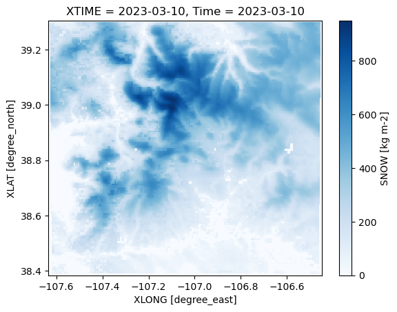
Investigate the change in SWE over time
first_ds = xr.open_dataset("../data/sail/wrf/wrfout_d03_2023-03-10_00_00_00").xwrf.postprocess().squeeze()
last_ds = xr.open_dataset("../data/sail/wrf/wrfout_d03_2023-03-11_00_00_00").xwrf.postprocess().squeeze()
Calculate the Change in SWE
Here, we take the difference using Xarray!
difference = last_ds["SNOW"] - first_ds["SNOW"]
last_ds["SNOW"]
<xarray.DataArray 'SNOW' (y: 201, x: 201)> Size: 162kB
[40401 values with dtype=float32]
Coordinates:
    XLAT     (y, x) float32 162kB 38.39 38.39 38.39 38.39 ... 39.3 39.3 39.3
    XLONG    (y, x) float32 162kB -107.6 -107.6 -107.6 ... -106.5 -106.5 -106.5
    XTIME    datetime64[ns] 8B ...
    CLAT     (y, x) float32 162kB 38.39 38.39 38.39 38.39 ... 39.3 39.3 39.3
    Time     datetime64[ns] 8B 2023-03-11
  * x        (x) float64 2kB -5.344e+04 -5.294e+04 ... 4.606e+04 4.656e+04
  * y        (y) float64 2kB -5.6e+04 -5.55e+04 -5.5e+04 ... 4.35e+04 4.4e+04
Attributes:
    FieldType:     104
    MemoryOrder:   XY
    description:   SNOW WATER EQUIVALENT
    units:         kg m-2
    stagger:
grid_mapping: wrf_projection- y: 201
- x: 201
- ...
[40401 values with dtype=float32]
- XLAT(y, x)float3238.39 38.39 38.39 ... 39.3 39.3
- FieldType :
- 104
- MemoryOrder :
- XY
- description :
- LATITUDE, SOUTH IS NEGATIVE
- units :
- degree_north
- stagger :
array([[38.38703 , 38.387066, 38.38709 , ..., 38.387497, 38.387466, 38.387444], [38.391594, 38.391624, 38.39166 , ..., 38.392063, 38.392033, 38.392006], [38.396156, 38.396194, 38.39622 , ..., 38.396633, 38.396603, 38.396572], ..., [39.290962, 39.290997, 39.291027, ..., 39.29144 , 39.291416, 39.291378], [39.29553 , 39.29556 , 39.295597, ..., 39.296005, 39.29598 , 39.295948], [39.3001 , 39.30013 , 39.300156, ..., 39.300564, 39.30055 , 39.300514]], dtype=float32) - XLONG(y, x)float32-107.6 -107.6 ... -106.5 -106.5
- FieldType :
- 104
- MemoryOrder :
- XY
- description :
- LONGITUDE, WEST IS NEGATIVE
- units :
- degree_east
- stagger :
array([[-107.62244 , -107.61661 , -107.610794, ..., -106.46942 , -106.46359 , -106.45778 ], [-107.62248 , -107.61667 , -107.61084 , ..., -106.46939 , -106.46356 , -106.45773 ], [-107.62253 , -107.6167 , -107.61087 , ..., -106.46936 , -106.46353 , -106.4577 ], ..., [-107.630646, -107.62474 , -107.618835, ..., -106.46243 , -106.45654 , -106.45062 ], [-107.63068 , -107.62479 , -107.61888 , ..., -106.4624 , -106.4565 , -106.45059 ], [-107.63072 , -107.62482 , -107.61893 , ..., -106.46237 , -106.45645 , -106.45056 ]], dtype=float32) - XTIME()datetime64[ns]...
- FieldType :
- 104
- MemoryOrder :
- 0
- description :
- minutes since 2021-09-15 00:00:00
- stagger :
[1 values with dtype=datetime64[ns]]
- CLAT(y, x)float3238.39 38.39 38.39 ... 39.3 39.3
- FieldType :
- 104
- MemoryOrder :
- XY
- description :
- COMPUTATIONAL GRID LATITUDE, SOUTH IS NEGATIVE
- units :
- degree_north
- stagger :
array([[38.38703 , 38.387066, 38.38709 , ..., 38.387497, 38.387466, 38.387444], [38.391594, 38.391624, 38.39166 , ..., 38.392063, 38.392033, 38.392006], [38.396156, 38.396194, 38.39622 , ..., 38.396633, 38.396603, 38.396572], ..., [39.290962, 39.290997, 39.291027, ..., 39.29144 , 39.291416, 39.291378], [39.29553 , 39.29556 , 39.295597, ..., 39.296005, 39.29598 , 39.295948], [39.3001 , 39.30013 , 39.300156, ..., 39.300564, 39.30055 , 39.300514]], dtype=float32) - Time()datetime64[ns]2023-03-11
- long_name :
- Time
- standard_name :
- time
array('2023-03-11T00:00:00.000000000', dtype='datetime64[ns]') - x(x)float64-5.344e+04 -5.294e+04 ... 4.656e+04
- units :
- m
- standard_name :
- projection_x_coordinate
- axis :
- X
array([-53443.825943, -52943.825943, -52443.825943, ..., 45556.174057, 46056.174057, 46556.174057]) - y(y)float64-5.6e+04 -5.55e+04 ... 4.4e+04
- units :
- m
- standard_name :
- projection_y_coordinate
- axis :
- Y
array([-55999.217634, -55499.217634, -54999.217634, ...,  43000.782366,
        43500.782366,  44000.782366])
- xPandasIndex
PandasIndex(Index([-53443.82594293087, -52943.82594293087, -52443.82594293087, -51943.82594293087, -51443.82594293087, -50943.82594293087, -50443.82594293087, -49943.82594293087, -49443.82594293087, -48943.82594293087, ... 42056.17405706913, 42556.17405706913, 43056.17405706913, 43556.17405706913, 44056.17405706913, 44556.17405706913, 45056.17405706913, 45556.17405706913, 46056.17405706913, 46556.17405706913], dtype='float64', name='x', length=201)) - yPandasIndex
PandasIndex(Index([-55999.217634373155, -55499.217634373155, -54999.217634373155,
       -54499.217634373155, -53999.217634373155, -53499.217634373155,
       -52999.217634373155, -52499.217634373155, -51999.217634373155,
       -51499.217634373155,
       ...
        39500.782365626845,  40000.782365626845,  40500.782365626845,
        41000.782365626845,  41500.782365626845,  42000.782365626845,
        42500.782365626845,  43000.782365626845,  43500.782365626845,
        44000.782365626845],
      dtype='float64', name='y', length=201))
- FieldType :
- 104
- MemoryOrder :
- XY
- description :
- SNOW WATER EQUIVALENT
- units :
- kg m-2
- stagger :
- grid_mapping :
- wrf_projection
difference.plot(x='XLONG',
                y='XLAT',
                cbar_kwargs={'label': "Change in Snow Water Equivalent ($kgm^{-2}$)"})
plt.title("24 Hour Difference in \n Snow Water Liquid Equivalent \n 10 March to 11 March 2023")
Text(0.5, 1.0, '24 Hour Difference in \n Snow Water Liquid Equivalent \n 10 March to 11 March 2023')
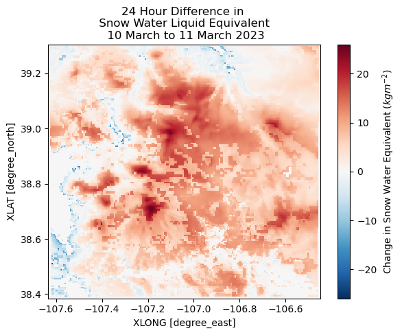
Challenge: Why is there more snow in some areas, and less in others?
Investigate other fields in the datasets
Look at other time steps - where are our precipitation fields?
Find possible scientific explanations here!
files = sorted(glob.glob("../data/sail/wrf/*"))
files
['../data/sail/wrf/wrfout_d03_2023-03-10_00_00_00',
 '../data/sail/wrf/wrfout_d03_2023-03-10_06_00_00',
 '../data/sail/wrf/wrfout_d03_2023-03-10_12_00_00',
 '../data/sail/wrf/wrfout_d03_2023-03-10_18_00_00',
 '../data/sail/wrf/wrfout_d03_2023-03-11_00_00_00']
Summary
xwrf can be a helpful tool when working with WRF data in Python! In this tutorial, we investigated WRF data from the SAIL campaign, digging into the datasets and using visualization techniques to analyze our results.
What’s next?
How do we scale up this analysis beyond a 24 hour run? Or higher resolution data? In future notebooks, we explore tools to help with increasing our ability to analyze high resolution datasets with xwrf.
Resources and references
This notebook was adapated from material in xwrf Documentation.
The dataset used here is an ARM PI dataset, courtesy of Zexuan Xu (zexuanxu@lbl.gov). If you use this dataset, please be sure to cite:
https://doi.org/10.5439/1971597
More information can be found in the related publication - https://doi.org/10.5194/egusphere-2022-437