Analyze microhh LES data

Contents

Analyze microhh LES data

In this notebook, we will analyze data from the microhh model, simulating a case near the Southern Great Plains.

Imports

#Load the usual libraries
import matplotlib.pyplot as plt
import xarray as xr
import scipy as sp
import numpy as np
import netCDF4 as nc

Find the Data

# locate the folder where the data is stored
basedir = '/data/project/ARM_Summer_School_2024_Data/summerschool_microhh/'
basename = 'SGP'
NC_arr = [10, 50, 80, 100, 200, 400, 800]

Configure some helper functions

# Load a specific data set, and cycling through all groups to load all data
def load_data(fname):
    groups = [''] + list(nc.Dataset(fname).groups.keys())
    prof_dict = {}
    for group in groups:
        try:
            prof_dict[group] = xr.open_dataset(fname, group=group, decode_times=True)
            
        except KeyError:
            print(f'Group {group} not found in {fname}')
        except IOError:
            print(f'File {fname} not found')
        except:
            print('Unexpected error')
    prof = xr.merge(prof_dict.values())
    prof = prof.where(prof.apply(np.fabs)<1e10)

    return prof

# Cycle through all conditional samples and load the data; the conditional sample is added as a new dimension
def load_cond_data(dir, basename, cond_samps):
    prof_dict = {}
    for cond_samp in cond_samps:
        fname = dir + '/' + basename +'.' + cond_samp + '.0000000.nc'
        prof_dict[cond_samp] = load_data(fname).expand_dims(dim={'sample': [cond_samp]})
    prof = xr.merge(prof_dict.values())
    return prof
    
# Cycle through all different Number concentrations and load the data; the number concentration is added as a new dimension
def load_all_data(basedir, fname, NCs, cond_samps = ['default']):
    prof_array = {}
    for NC in NCs:
        NCstr = f'NC{NC:03}'
        print('Loading data for ' + NCstr)
        dir = basedir + '/' + NCstr + '/'
        prof_array[NCstr] = load_cond_data(dir, basename, cond_samps).expand_dims(dim={'NC': [NC]})

    return xr.merge(prof_array.values())

Run through the Analysis

# Load the data for all number concentrations and conditional samples
cond_samps = ['default', 'ql', 'qlcore']
prof = load_all_data(basedir, basename, NC_arr, cond_samps)

#Slice the data for our area of interest, and resample to 30 min intervals
prof = prof.sel(time=slice("2016-06-11T12", "2016-06-12T02"),z=slice(0,4000), zh=slice(0,4000)).resample(time='0.5H').mean(dim='time')

Loading data for NC010
Loading data for NC050
Loading data for NC080
Loading data for NC100
Loading data for NC200
Loading data for NC400
Loading data for NC800

# We first explore a few basic statistics, such as overall cloud cover, LWP, cloud base height, and cloud top height
plt.figure()
prof.sel(NC=100, sample='default')['ql_cover'].plot()

plt.figure()
prof.sel(NC=100, sample='default')['ql_path'].plot()

plt.figure()
prof.sel(NC=100, sample='default')['qr_path'].plot()

[<matplotlib.lines.Line2D at 0x7f7fc0ca8e80>]

../../_images/e7f7868a80baf798a6e11fa125e6757e834b31873e55168f06cd0bfddb862d00.png

../../_images/1841c3c339d91c30b5babea2f6ee4f595e46973c5d54715ab11a742557c830ee.png

../../_images/e4cec1efd45ddeb5a18d793979464958be0681024feaf8c36d7b8504cb077c93.png

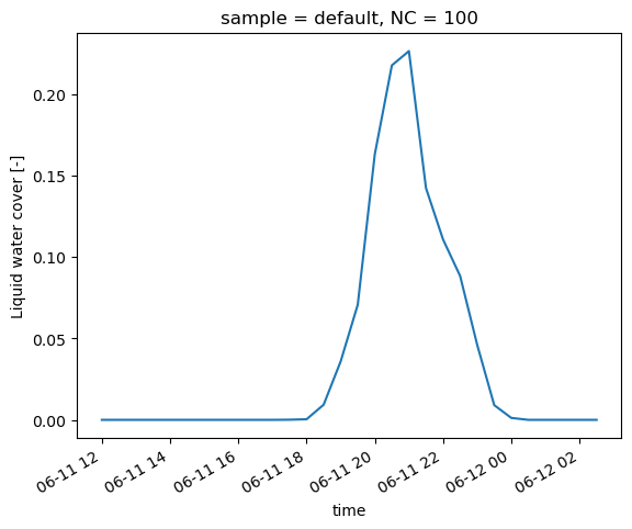
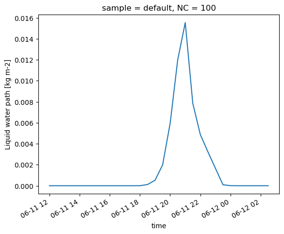
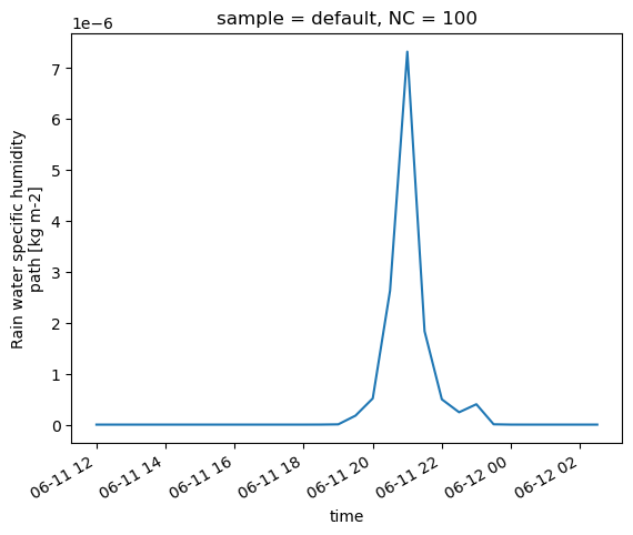
prof.sel(NC=100, sample='default')['ql'].where(prof.sel(NC=100, sample='default').ql>0).plot(x='time')

<matplotlib.collections.QuadMesh at 0x7f7fc0b5bd30>

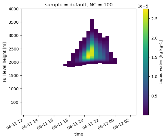
../../_images/a6113c860189818e0944fda83c93061a1569600c6472b4e84cf1fd8957a5d5d7.png

 #At 22:00, we are at peak cloudiness. Let's explore the vertical structure of the cloud at this time
 plt.figure()
 prof.sel(time='2016-06-11T22:00', NC=100).thl.plot.line(y='z', hue='sample')
 plt.figure()
 prof.sel(time='2016-06-11T22:00', NC=100).qt.plot.line(y='z', hue='sample')
 plt.figure()
 prof.sel(time='2016-06-11T22:00', NC=100).w.plot.line(y='zh', hue='sample')

[<matplotlib.lines.Line2D at 0x7f7fc0ad2b60>,
 <matplotlib.lines.Line2D at 0x7f7fc0ad2b00>,
 <matplotlib.lines.Line2D at 0x7f7fc0ad2d10>]

../../_images/43455fea459e4fc66c651a839d2429c178ec465a5662f564137773d05531a63f.png

../../_images/f439f747614515209be4566b7fc34062c1443eb8d7039c6d22d59bccf98e44c9.png

../../_images/b86ce79cd97d01bfb10efa421c3a029954212d4893d20cc8704cdef16363fc02.png

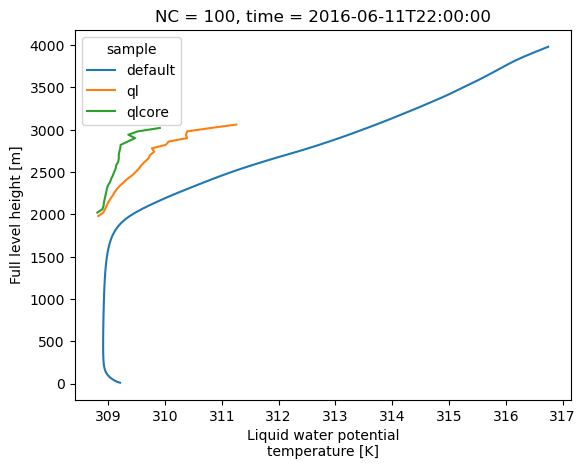
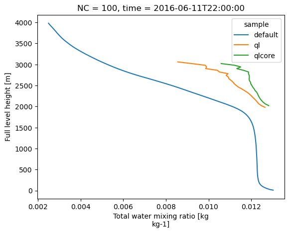
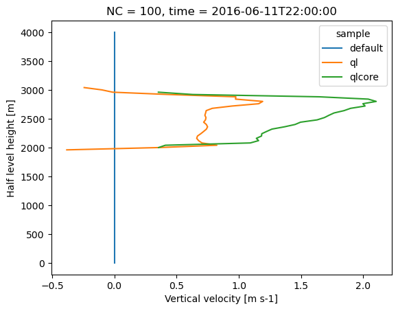
#Now for the moisture flux: Is this correct??
prof.sel(sample='default', NC=100, time="2016-06-11T22:00").qt_w.plot(y='zh')

#We should not forget to add the Sub Filter Scale Fluxes; the MicroHH output has that automatically as '_flux'. What do you notice about the following plot?
prof.sel(sample='default', NC=100, time="2016-06-11T22:00").qt_w.plot(y='zh')
prof.sel(sample='default', NC=100, time="2016-06-11T22:00").qt_diff.plot(y='zh')
prof.sel(sample='default', NC=100, time="2016-06-11T22:00").qt_flux.plot(y='zh')

[<matplotlib.lines.Line2D at 0x7f7fc05f63e0>]

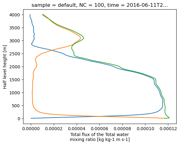
../../_images/9ff4636b0ccbf8f2c0dfced16894158b8139861f242a9d4677e87cea3f7905cb.png

# Calculate the cloud base and cloud top heights, that is, the first and last point where the liquid water content is larger than zero
prof['cb'] = (prof['ql']>0).idxmax(dim='z')
prof['cb'] = prof.cb.where(prof.cb>prof.z[0]) # remove cloud base if they are at the lowest level 

prof['ct'] = (prof['ql']>0).isel(z=slice(None, None, -1)).idxmax(dim='z')
prof['ct'] = prof.ct.where(prof.ct<prof.z[-1]) # remove cloud top if they are at the highest level

# Plot them
prof.sel(sample='default')['cb'].plot.line(hue='NC')
prof.sel(sample='default')['ct'].plot.line(hue='NC')
# prof.sel(sample='default')['ct'].plot()

[<matplotlib.lines.Line2D at 0x7f7fc065b310>,
 <matplotlib.lines.Line2D at 0x7f7fc065b340>,
 <matplotlib.lines.Line2D at 0x7f7fc065b0d0>,
 <matplotlib.lines.Line2D at 0x7f7fc062dde0>,
 <matplotlib.lines.Line2D at 0x7f7fc065ad10>,
 <matplotlib.lines.Line2D at 0x7f7fc0659300>,
 <matplotlib.lines.Line2D at 0x7f7fc0659f30>]

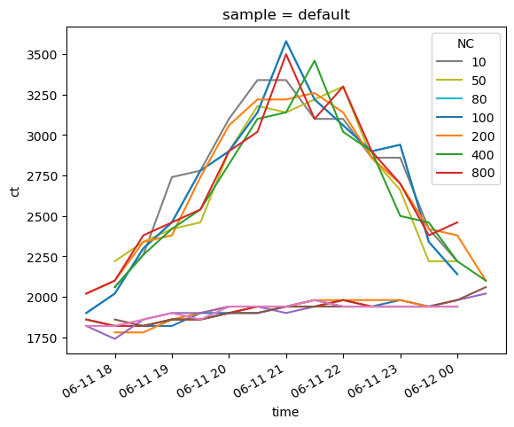
../../_images/784e486ca3ee8624983e6df5abdb548f25ab339439ab2ce277cfcd6b46e553e2.png

prof.sel(sample='ql').ql.plot(x='time', col='NC', col_wrap=4)

<xarray.plot.facetgrid.FacetGrid at 0x7f7fc5afbe50>

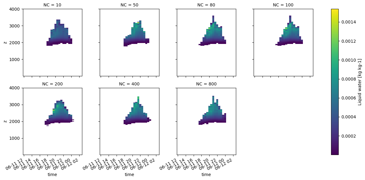
../../_images/a66d97790c9847228ce9b44def3d6962f460c9fb92cefe77a83dd80c2d850850.png

(-prof.sel(sample='default').qr_flux.sel(zh=0).cumsum()).plot(x='time', hue='NC')

[<matplotlib.lines.Line2D at 0x7f7fc10fbfa0>,
 <matplotlib.lines.Line2D at 0x7f7fc0f21030>,
 <matplotlib.lines.Line2D at 0x7f7fc0f20ee0>,
 <matplotlib.lines.Line2D at 0x7f7fc0f20e20>,
 <matplotlib.lines.Line2D at 0x7f7fc10bb8e0>,
 <matplotlib.lines.Line2D at 0x7f7fc10bb910>,
 <matplotlib.lines.Line2D at 0x7f7fc0f21210>]

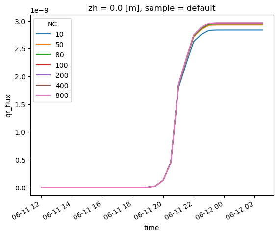
../../_images/bc1e3e79dbe7e94040428e6cfe1a0431d15e2b6ac133d7fdb6f9c342ced245e1.png

#Bulk entrainment is defined as \epsilon = -\frac{d\theta_l}{dz} / (\phi_c - \phi_e), where \phi_c is the cloud property, and \phi_e are the environmental properties.
#We will use the cloud potential temperature as the cloud property, and the environmental potential temperature as the environmental property
epsilon = prof.sel(time='2016-06-11T22:00', sample='ql').thl.differentiate(coord='z') / (prof.sel(time='2016-06-11T22:00', sample='default').thl - prof.sel(time='2016-06-11T22:00', sample='ql').thl)
epsilon.plot.line(y='z', hue='NC')

[<matplotlib.lines.Line2D at 0x7f7fc06c6e90>,
 <matplotlib.lines.Line2D at 0x7f7fc06c6e30>,
 <matplotlib.lines.Line2D at 0x7f7fc06c7040>,
 <matplotlib.lines.Line2D at 0x7f7fc06c7160>,
 <matplotlib.lines.Line2D at 0x7f7fc06c7280>,
 <matplotlib.lines.Line2D at 0x7f7fc06c73a0>,
 <matplotlib.lines.Line2D at 0x7f7fc06c74c0>]

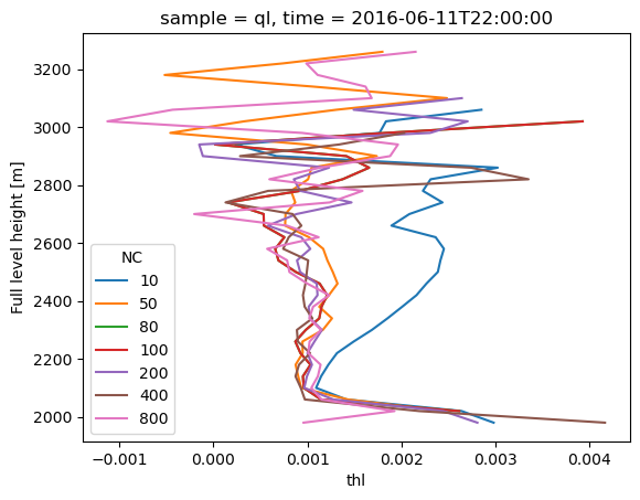
../../_images/9ecdc3602eee3b2d502982f6ee4f92aedfeedda14c652b23e223b723299cbfe2.png

prof.sel(sample='default', NC=100, time="2016-06-11T22:00").qt_w.plot(y='zh')
prof.sel(sample='default', NC=100, time="2016-06-11T22:00").qt_diff.plot(y='zh')
prof.sel(sample='default', NC=100, time="2016-06-11T22:00").qt_flux.plot(y='zh')

[<matplotlib.lines.Line2D at 0x7f7604c2b3a0>]

../../_images/9ff4636b0ccbf8f2c0dfced16894158b8139861f242a9d4677e87cea3f7905cb.png

prof.sel(sample='default').ql_cover.plot(x='time', hue='NC')

[<matplotlib.lines.Line2D at 0x7f76046334c0>,
 <matplotlib.lines.Line2D at 0x7f7604662ef0>,
 <matplotlib.lines.Line2D at 0x7f7604662da0>,
 <matplotlib.lines.Line2D at 0x7f7604662ce0>,
 <matplotlib.lines.Line2D at 0x7f7604662fb0>,
 <matplotlib.lines.Line2D at 0x7f76046630d0>,
 <matplotlib.lines.Line2D at 0x7f76046631f0>,
 <matplotlib.lines.Line2D at 0x7f7604663310>]

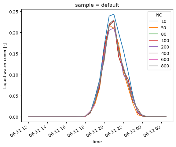
../../_images/1e5b82d553d0bc45a88b63b814b8210864308d14fa36011ab3aae625bbd804f8.png

plt.figure()
prof.sel(sample='default', time="2016-06-11T22:00").qt_flux.plot(y='zh', hue='NC')

plt.figure()
prof.sel(sample='default', time="2016-06-11T22:00").thl_flux.plot(y='zh', hue='NC')

[<matplotlib.lines.Line2D at 0x7f7fc04b8e50>,
 <matplotlib.lines.Line2D at 0x7f7fc04b8df0>,
 <matplotlib.lines.Line2D at 0x7f7fc04b9000>,
 <matplotlib.lines.Line2D at 0x7f7fc04b9120>,
 <matplotlib.lines.Line2D at 0x7f7fc04b9240>,
 <matplotlib.lines.Line2D at 0x7f7fc04b9360>,
 <matplotlib.lines.Line2D at 0x7f7fc04b9480>]

../../_images/23b679085632eeb162445fd5aff3d28f9a7b431e4bab179bf80190effe66450a.png

../../_images/dd2595581d841db74426e4f6f7b7d2d75fa82a6172c3a5ecfa67435da93d89f7.png