Overview of LASSO-ShCu Data for Southern Great Plains
The LASSO Shallow-Convection scenario focuses on shallow convective clouds at the Southern Great Plains (SGP) atmospheric obesrvatory in Oklahoma. Ensembles of idealized large-eddy simulation (LES) runs are available for 95 case dates spanning the years 2015-2019.
Useful links for more information:
Author: William.Gustafson@pnnl.gov
Date: 10-May-2024
# Libraries required for this tutorial...

# import dask
from datetime import datetime
import numpy as np
import xarray as xr
import xwrf

import matplotlib.pyplot as plt
Avaialble LASSO-ShCu Datastreams
LASSO-ShCu consists of a suite of datastreams that combine a library of LES simulations with ARM observations to put the simulations in the context of reality for each case date. The following datastreams can be downloaded from the :
sgplassodiagconfobsmod: Config-Obs-Model
Input data necessary to reproduce a simulation
Skill score information and plots summarizing model results for each simulation in the case date’s ensemble, typically hourly resolution
sgplassodiagraw: Raw Model Output
wrfouthourly files containing instantaenous model snapshots every 10 minuteswrfstatfiles containing LES statistics every 10 minutes, e.g., output-period-averaged domain-mean profiles
sgplassocogsdiagobsmod: Clouds Optically Gridded by Stereo (COGS)-based skill analysis; when avaialble (only 2018-2019), this is considered more reliable than the ARSCL-based skill-scores for cloud fraction in
sgplassodiagconfobsmod1-minute and 10-minute sampled cloud fraction obserations using COGS
Overview cloud-fraction skill-score values and plots for the simulation ensemble for the selected case date
Simulation-specific cloud-fraction skill-score information for each simulation on the selected case date
sgplassohighfreqobs: High-frequency observations that were used to build
sgplassodiagconfobsmodsgp915rwpwindcon10mC1.c1: Wind profiles retrieved from radar-wind profilers at C1, I8, I9, and I10, 10-minute intervals
sgpcldfracset*C1.c1: KAZR-ARSCL derived time-height cloud fraction profiles for 1, 5, and 15-minute intervals
sgplassoblthermoC1.c1: Boundary-layer thermodynamic information for 500-700 m above surface from AERIoe and Raman lidar retrievals; temperature, water vapor mixing ratio, relative humidity, and pressure on 10-minute interval
sgplassodlcbhshcu*.c1: cloud-base height from Doppler lidar at stations C1, E32, E37, E39, and E41
sgplassolwpC1.c1: Liquid water path retrieved from AERI and MWRRET
sgplclC1.c1: Lifting condensation level for meteorology stations in the Oklahoma region
Downloading and Organizing the Datastreams
All of the above datastreams can be downloaded from the LASSO-ShCu bundle Browser. The table at the bottom of that webpage updates based on selections made in the checkboxes along the lefthand side of the page. Then, one selects which simulations and associated files are desired within the table. When all selections have been made, the Order Data button is at the bottom of the page. Users will have the most reliable download experience by also turning on the Globus option within Download Options. Most of the datastreams are managemable, with the exception of sgplassodiagraw, which can be a bit large for some users to work with–that one can crash FTP downloads via html and Globus gets around this issue.
Some datastreams contain files just for one simulation, while others have multiple simulations worth of information. So, the folder structures within the datastreams varies. An easy way to organize the data is in a tree structure by case date and simulation ID. This can be done by placing downloaded tar files into a single folder and then running support_code/stage_lasso_shcu-data.py that is in this tutorial’s sub-folder.
The remainder of this notebook assumes one is working with data organized using stage_lasso_shcu_data.py.
Raw WRF Output from LASSO-ShCu
The core of LASSO-ShCu is raw simulation output from the Weather Research and Forecasting (WRF) model, which has been run in an idealized LES mode with doubly periodic boundaries. The traditional wrfout file from WRF is provided to the users as-is. The bulk of the variables within the file are as one would expect from WRF. Additionaly, some LES-specific information is output, such as the forcing tendencies. LES modelers frequently work with summary statistics instead of cell-by-cell data, so we also output a wrfstat file that provides 10-minute averages for various metorology variables and diagnostics. Diagnostics include variables like cloud and ice water paths, domain-averaged profiles, fluxes, and in-cloud statistics.
Let’s take a look at a wrfstat file first since these are smaller and easier to work with.
# Plotting wrfstat variables...

# path_shcu_root = "/gpfs/wolf2/arm/atm124/world-shared/arm-summer-school-2024/lasso_tutorial/ShCu/untar/"  # on cumulus
path_shcu_root = "/data/project/ARM_Summer_School_2024_Data/lasso_tutorial/ShCu/untar"  # on Jupyter

case_date = datetime(2019, 4, 4)
sim_id = 4

ds_stat = xr.open_dataset(f"{path_shcu_root}/{case_date:%Y%m%d}/sim{sim_id:04d}/raw_model/wrfstat_d01_{case_date:%Y-%m-%d_12:00:00}.nc")
ds_stat
ERROR 1: PROJ: proj_create_from_database: Open of /opt/conda/share/proj failed
<xarray.Dataset> Size: 72GB
Dimensions:         (Time: 91, bottom_top: 226, bottom_top_stag: 227,
                     south_north: 250, west_east: 250, west_east_stag: 251,
                     south_north_stag: 251)
Coordinates:
    XTIME           (Time) datetime64[ns] 728B ...
Dimensions without coordinates: Time, bottom_top, bottom_top_stag, south_north,
                                west_east, west_east_stag, south_north_stag
Data variables: (12/179)
    Times           (Time) |S19 2kB ...
    CST_CLDLOW      (Time) float32 364B ...
    CST_CLDTOT      (Time) float32 364B ...
    CST_LWP         (Time) float32 364B ...
    CST_IWP         (Time) float32 364B ...
    CST_PRECW       (Time) float32 364B ...
    ...              ...
    CSV_IWC         (Time, bottom_top, south_north, west_east) float32 5GB ...
    CSV_CLDFRAC     (Time, bottom_top, south_north, west_east) float32 5GB ...
    CSS_LWP         (Time, south_north, west_east) float32 23MB ...
    CSS_IWP         (Time, south_north, west_east) float32 23MB ...
    CSS_CLDTOT      (Time, south_north, west_east) float32 23MB ...
    CSS_CLDLOW      (Time, south_north, west_east) float32 23MB ...
Attributes: (12/96)
    TITLE:                                  OUTPUT FROM WRF V3.8.1 MODEL
    START_DATE:                            2019-04-04_12:00:00
    WEST-EAST_GRID_DIMENSION:              251
    SOUTH-NORTH_GRID_DIMENSION:            251
    BOTTOM-TOP_GRID_DIMENSION:             227
    DX:                                    100.0
    ...                                    ...
    config_aerosol:                        NA
    config_forecast_time:                  15.0 h
    config_boundary_method:                Periodic
    config_microphysics:                   Thompson (mp_physics=8)
    config_nickname:                       runlas20190404v1addhm
simulation_origin_host: cumulus-login2.ccs.ornl.gov- Time: 91
- bottom_top: 226
- bottom_top_stag: 227
- south_north: 250
- west_east: 250
- west_east_stag: 251
- south_north_stag: 251
- XTIME(Time)datetime64[ns]...
- FieldType :
- 104
- MemoryOrder :
- 0
- description :
- minutes since 2019-04-04 12:00:00
- stagger :
[91 values with dtype=datetime64[ns]]
- Times(Time)|S19...
[91 values with dtype=|S19]
- CST_CLDLOW(Time)float32...
- FieldType :
- 104
- MemoryOrder :
- 0
- description :
- Fractional low-cloud cover (<5 km)
- units :
- (0-1)
- stagger :
[91 values with dtype=float32]
- CST_CLDTOT(Time)float32...
- FieldType :
- 104
- MemoryOrder :
- 0
- description :
- Fractional cloud cover
- units :
- (0-1)
- stagger :
[91 values with dtype=float32]
- CST_LWP(Time)float32...
- FieldType :
- 104
- MemoryOrder :
- 0
- description :
- Vertical integrated liquid water path (based on ql)
- units :
- kg/m^2
- stagger :
[91 values with dtype=float32]
- CST_IWP(Time)float32...
- FieldType :
- 104
- MemoryOrder :
- 0
- description :
- Vertical integrated ice water path (based on qf)
- units :
- kg/m^2
- stagger :
[91 values with dtype=float32]
- CST_PRECW(Time)float32...
- FieldType :
- 104
- MemoryOrder :
- 0
- description :
- Vertical integrated water vapor
- units :
- kg/m^2
- stagger :
[91 values with dtype=float32]
- CST_TKE(Time)float32...
- FieldType :
- 104
- MemoryOrder :
- 0
- description :
- Vertical integrated TKE
- units :
- kg/s^2
- stagger :
[91 values with dtype=float32]
- CST_TSAIR(Time)float32...
- FieldType :
- 104
- MemoryOrder :
- 0
- description :
- Surface air temperature
- units :
- K
- stagger :
[91 values with dtype=float32]
- CST_PS(Time)float32...
- FieldType :
- 104
- MemoryOrder :
- 0
- description :
- Surface pressure
- units :
- Pa
- stagger :
[91 values with dtype=float32]
- CST_PRECT(Time)float32...
- FieldType :
- 104
- MemoryOrder :
- 0
- description :
- Total precipitation at surface
- units :
- mm/sec
- stagger :
[91 values with dtype=float32]
- CST_SH(Time)float32...
- FieldType :
- 104
- MemoryOrder :
- 0
- description :
- Surface sensible heat flux
- units :
- W/m^2
- stagger :
[91 values with dtype=float32]
- CST_LH(Time)float32...
- FieldType :
- 104
- MemoryOrder :
- 0
- description :
- Surface latent heat flux
- units :
- W/m^2
- stagger :
[91 values with dtype=float32]
- CST_FSNTC(Time)float32...
- FieldType :
- 104
- MemoryOrder :
- 0
- description :
- TOA SW net upward clear-sky radiation
- units :
- W/m^2
- stagger :
[91 values with dtype=float32]
- CST_FSNT(Time)float32...
- FieldType :
- 104
- MemoryOrder :
- 0
- description :
- TOA SW net upward total-sky radiation
- units :
- W/m^2
- stagger :
[91 values with dtype=float32]
- CST_FLNTC(Time)float32...
- FieldType :
- 104
- MemoryOrder :
- 0
- description :
- TOA LW (net) upward clear-sky radiation
- units :
- W/m^2
- stagger :
[91 values with dtype=float32]
- CST_FLNT(Time)float32...
- FieldType :
- 104
- MemoryOrder :
- 0
- description :
- TOA LW (net) upward total-sky radiation
- units :
- W/m^2
- stagger :
[91 values with dtype=float32]
- CST_FSNSC(Time)float32...
- FieldType :
- 104
- MemoryOrder :
- 0
- description :
- Surface SW net upward clear-sky radiation
- units :
- W/m^2
- stagger :
[91 values with dtype=float32]
- CST_FSNS(Time)float32...
- FieldType :
- 104
- MemoryOrder :
- 0
- description :
- Surface SW net upward total-sky radiation
- units :
- W/m^2
- stagger :
[91 values with dtype=float32]
- CST_FLNSC(Time)float32...
- FieldType :
- 104
- MemoryOrder :
- 0
- description :
- Surface LW net upward clear-sky radiation
- units :
- W/m^2
- stagger :
[91 values with dtype=float32]
- CST_FLNS(Time)float32...
- FieldType :
- 104
- MemoryOrder :
- 0
- description :
- Surface LW net upward total-sky radiation
- units :
- W/m^2
- stagger :
[91 values with dtype=float32]
- CST_SWINC(Time)float32...
- FieldType :
- 104
- MemoryOrder :
- 0
- description :
- TOA solar insolation
- units :
- W/m^2
- stagger :
[91 values with dtype=float32]
- CST_TSK(Time)float32...
- FieldType :
- 104
- MemoryOrder :
- 0
- description :
- Surface skin temperature
- units :
- K
- stagger :
[91 values with dtype=float32]
- CST_UST(Time)float32...
- FieldType :
- 104
- MemoryOrder :
- 0
- description :
- Surface friction velocity
- units :
- m/s
- stagger :
[91 values with dtype=float32]
- CSP_Z(Time, bottom_top)float32...
- FieldType :
- 104
- MemoryOrder :
- Z
- description :
- Half level height
- units :
- m
- stagger :
[20566 values with dtype=float32]
- CSP_Z8W(Time, bottom_top_stag)float32...
- FieldType :
- 104
- MemoryOrder :
- Z
- description :
- Full level height
- units :
- m
- stagger :
- Z
[20657 values with dtype=float32]
- CSP_DZ8W(Time, bottom_top)float32...
- FieldType :
- 104
- MemoryOrder :
- Z
- description :
- dz at full level
- units :
- m
- stagger :
[20566 values with dtype=float32]
- CSP_U(Time, bottom_top)float32...
- FieldType :
- 104
- MemoryOrder :
- Z
- description :
- Zonal wind
- units :
- m/s
- stagger :
[20566 values with dtype=float32]
- CSP_V(Time, bottom_top)float32...
- FieldType :
- 104
- MemoryOrder :
- Z
- description :
- Meridional wind
- units :
- m/s
- stagger :
[20566 values with dtype=float32]
- CSP_W(Time, bottom_top_stag)float32...
- FieldType :
- 104
- MemoryOrder :
- Z
- description :
- Vertical motion
- units :
- m/s
- stagger :
- Z
[20657 values with dtype=float32]
- CSP_P(Time, bottom_top)float32...
- FieldType :
- 104
- MemoryOrder :
- Z
- description :
- Pressure
- units :
- Pa
- stagger :
[20566 values with dtype=float32]
- CSP_TH(Time, bottom_top)float32...
- FieldType :
- 104
- MemoryOrder :
- Z
- description :
- Potential temperature
- units :
- K
- stagger :
[20566 values with dtype=float32]
- CSP_THV(Time, bottom_top)float32...
- FieldType :
- 104
- MemoryOrder :
- Z
- description :
- Virtual potential temperature
- units :
- K
- stagger :
[20566 values with dtype=float32]
- CSP_THL(Time, bottom_top)float32...
- FieldType :
- 104
- MemoryOrder :
- Z
- description :
- Liquid water potential temperature
- units :
- K
- stagger :
[20566 values with dtype=float32]
- CSP_QV(Time, bottom_top)float32...
- FieldType :
- 104
- MemoryOrder :
- Z
- description :
- Water vapor mixing ratio
- units :
- kg/kg
- stagger :
[20566 values with dtype=float32]
- CSP_QC(Time, bottom_top)float32...
- FieldType :
- 104
- MemoryOrder :
- Z
- description :
- Cloud water mixing ratio
- units :
- kg/kg
- stagger :
[20566 values with dtype=float32]
- CSP_QI(Time, bottom_top)float32...
- FieldType :
- 104
- MemoryOrder :
- Z
- description :
- Ice crystal (cloud ice) mixing ratio
- units :
- kg/kg
- stagger :
[20566 values with dtype=float32]
- CSP_QL(Time, bottom_top)float32...
- FieldType :
- 104
- MemoryOrder :
- Z
- description :
- Liquid water mixing ratio
- units :
- kg/kg
- stagger :
[20566 values with dtype=float32]
- CSP_QF(Time, bottom_top)float32...
- FieldType :
- 104
- MemoryOrder :
- Z
- description :
- Frozen water mixing ratio
- units :
- kg/kg
- stagger :
[20566 values with dtype=float32]
- CSP_QT(Time, bottom_top)float32...
- FieldType :
- 104
- MemoryOrder :
- Z
- description :
- Total (vapor+liquid+frozen) water mixing ratio
- units :
- kg/kg
- stagger :
[20566 values with dtype=float32]
- CSP_LWC(Time, bottom_top)float32...
- FieldType :
- 104
- MemoryOrder :
- Z
- description :
- Liquid water content (based on ql)
- units :
- kg/m^3
- stagger :
[20566 values with dtype=float32]
- CSP_IWC(Time, bottom_top)float32...
- FieldType :
- 104
- MemoryOrder :
- Z
- description :
- Ice water content (based on qf)
- units :
- kg/m^3
- stagger :
[20566 values with dtype=float32]
- CSP_SPEQV(Time, bottom_top)float32...
- FieldType :
- 104
- MemoryOrder :
- Z
- description :
- Specific humidity
- units :
- kg/kg
- stagger :
[20566 values with dtype=float32]
- CSP_A_CL(Time, bottom_top)float32...
- FieldType :
- 104
- MemoryOrder :
- Z
- description :
- Fraction of cloudy grid points
- units :
- (0-1)
- stagger :
[20566 values with dtype=float32]
- CSP_RHO(Time, bottom_top)float32...
- FieldType :
- 104
- MemoryOrder :
- Z
- description :
- Density
- units :
- kg/m^3
- stagger :
[20566 values with dtype=float32]
- CSP_U2(Time, bottom_top)float32...
- FieldType :
- 104
- MemoryOrder :
- Z
- description :
- u_p^2
- units :
- m^2/s^2
- stagger :
[20566 values with dtype=float32]
- CSP_V2(Time, bottom_top)float32...
- FieldType :
- 104
- MemoryOrder :
- Z
- description :
- v_p^2
- units :
- m^2/s^2
- stagger :
[20566 values with dtype=float32]
- CSP_U2V2(Time, bottom_top)float32...
- FieldType :
- 104
- MemoryOrder :
- Z
- description :
- u_p^2+v_p^2
- units :
- m^2/s^2
- stagger :
[20566 values with dtype=float32]
- CSP_W2(Time, bottom_top_stag)float32...
- FieldType :
- 104
- MemoryOrder :
- Z
- description :
- w_p^2
- units :
- m^2/s^2
- stagger :
- Z
[20657 values with dtype=float32]
- CSP_W3(Time, bottom_top_stag)float32...
- FieldType :
- 104
- MemoryOrder :
- Z
- description :
- w_p^3
- units :
- m^3/s^3
- stagger :
- Z
[20657 values with dtype=float32]
- CSP_WSKEW(Time, bottom_top_stag)float32...
- FieldType :
- 104
- MemoryOrder :
- Z
- description :
- Skewness <w3>/<w2>^(3/2)
- units :
- stagger :
- Z
[20657 values with dtype=float32]
- CSP_UW(Time, bottom_top)float32...
- FieldType :
- 104
- MemoryOrder :
- Z
- description :
- x-momentum flux uw (rs+sgs)
- units :
- m^2/s^2
- stagger :
[20566 values with dtype=float32]
- CSP_VW(Time, bottom_top)float32...
- FieldType :
- 104
- MemoryOrder :
- Z
- description :
- y-momentum flux vw (rs+sgs)
- units :
- m^2/s^2
- stagger :
[20566 values with dtype=float32]
- CSP_WTH(Time, bottom_top)float32...
- FieldType :
- 104
- MemoryOrder :
- Z
- description :
- Potential temperature flux (rs+sgs)
- units :
- K m/s
- stagger :
[20566 values with dtype=float32]
- CSP_WTHV(Time, bottom_top)float32...
- FieldType :
- 104
- MemoryOrder :
- Z
- description :
- Virtual potential temperature flux (rs+sgs)
- units :
- K m/s
- stagger :
[20566 values with dtype=float32]
- CSP_WTHL(Time, bottom_top)float32...
- FieldType :
- 104
- MemoryOrder :
- Z
- description :
- Liquid water potential temperature flux (rs+sgs)
- units :
- K m/s
- stagger :
[20566 values with dtype=float32]
- CSP_WQV(Time, bottom_top)float32...
- FieldType :
- 104
- MemoryOrder :
- Z
- description :
- Water vapor flux (rs+sgs)
- units :
- kg/kg m/s
- stagger :
[20566 values with dtype=float32]
- CSP_WQC(Time, bottom_top)float32...
- FieldType :
- 104
- MemoryOrder :
- Z
- description :
- Cloud water flux (rs+sgs)
- units :
- kg/kg m/s
- stagger :
[20566 values with dtype=float32]
- CSP_WQI(Time, bottom_top)float32...
- FieldType :
- 104
- MemoryOrder :
- Z
- description :
- Ice crystal (cloud ice) flux (rs+sgs)
- units :
- kg/kg m/s
- stagger :
[20566 values with dtype=float32]
- CSP_WQL(Time, bottom_top)float32...
- FieldType :
- 104
- MemoryOrder :
- Z
- description :
- Liquid water flux (rs+sgs)
- units :
- kg/kg m/s
- stagger :
[20566 values with dtype=float32]
- CSP_WQF(Time, bottom_top)float32...
- FieldType :
- 104
- MemoryOrder :
- Z
- description :
- Frozen water flux (rs+sgs)
- units :
- kg/kg m/s
- stagger :
[20566 values with dtype=float32]
- CSP_WQT(Time, bottom_top)float32...
- FieldType :
- 104
- MemoryOrder :
- Z
- description :
- Total water flux (rs+sgs)
- units :
- kg/kg m/s
- stagger :
[20566 values with dtype=float32]
- CSP_UW_SGS(Time, bottom_top)float32...
- FieldType :
- 104
- MemoryOrder :
- Z
- description :
- x-momentum flux uw (sgs)
- units :
- m^2/s^2
- stagger :
[20566 values with dtype=float32]
- CSP_VW_SGS(Time, bottom_top)float32...
- FieldType :
- 104
- MemoryOrder :
- Z
- description :
- y-momentum flux vw (sgs)
- units :
- m^2/s^2
- stagger :
[20566 values with dtype=float32]
- CSP_WTH_SGS(Time, bottom_top)float32...
- FieldType :
- 104
- MemoryOrder :
- Z
- description :
- Potential temperature flux (sgs)
- units :
- K m/s
- stagger :
[20566 values with dtype=float32]
- CSP_WTHV_SGS(Time, bottom_top)float32...
- FieldType :
- 104
- MemoryOrder :
- Z
- description :
- Virtual potential temperature flux (sgs)
- units :
- K m/s
- stagger :
[20566 values with dtype=float32]
- CSP_WTHL_SGS(Time, bottom_top)float32...
- FieldType :
- 104
- MemoryOrder :
- Z
- description :
- Liquid water potential temperature flux (sgs)
- units :
- K m/s
- stagger :
[20566 values with dtype=float32]
- CSP_WQV_SGS(Time, bottom_top)float32...
- FieldType :
- 104
- MemoryOrder :
- Z
- description :
- Water vapor flux (sgs)
- units :
- kg/kg m/s
- stagger :
[20566 values with dtype=float32]
- CSP_WQC_SGS(Time, bottom_top)float32...
- FieldType :
- 104
- MemoryOrder :
- Z
- description :
- Cloud water flux (sgs)
- units :
- kg/kg m/s
- stagger :
[20566 values with dtype=float32]
- CSP_WQI_SGS(Time, bottom_top)float32...
- FieldType :
- 104
- MemoryOrder :
- Z
- description :
- Ice crystal (cloud ice) flux (sgs)
- units :
- kg/kg m/s
- stagger :
[20566 values with dtype=float32]
- CSP_WQL_SGS(Time, bottom_top)float32...
- FieldType :
- 104
- MemoryOrder :
- Z
- description :
- Liquid water flux (sgs)
- units :
- kg/kg m/s
- stagger :
[20566 values with dtype=float32]
- CSP_WQF_SGS(Time, bottom_top)float32...
- FieldType :
- 104
- MemoryOrder :
- Z
- description :
- Frozen water flux (sgs)
- units :
- kg/kg m/s
- stagger :
[20566 values with dtype=float32]
- CSP_WQT_SGS(Time, bottom_top)float32...
- FieldType :
- 104
- MemoryOrder :
- Z
- description :
- Total water flux (sgs)
- units :
- kg/kg m/s
- stagger :
[20566 values with dtype=float32]
- CSP_SEDFQC(Time, bottom_top)float32...
- FieldType :
- 104
- MemoryOrder :
- Z
- description :
- Sedimentation flux of qc
- units :
- kg /m^2/s
- stagger :
[20566 values with dtype=float32]
- CSP_SEDFQR(Time, bottom_top)float32...
- FieldType :
- 104
- MemoryOrder :
- Z
- description :
- Sedimentation (Precipitation) flux of qr
- units :
- kg /m^2/s
- stagger :
[20566 values with dtype=float32]
- CSP_THDT_COND(Time, bottom_top)float32...
- FieldType :
- 104
- MemoryOrder :
- Z
- description :
- dth/dt due to net condensation
- units :
- K/s
- stagger :
[20566 values with dtype=float32]
- CSP_THDT_LW(Time, bottom_top)float32...
- FieldType :
- 104
- MemoryOrder :
- Z
- description :
- dth/dt due to LW radiation
- units :
- K/s
- stagger :
[20566 values with dtype=float32]
- CSP_THDT_SW(Time, bottom_top)float32...
- FieldType :
- 104
- MemoryOrder :
- Z
- description :
- dth/dt due to SW radiation
- units :
- K/s
- stagger :
[20566 values with dtype=float32]
- CSP_THDT_LS(Time, bottom_top)float32...
- FieldType :
- 104
- MemoryOrder :
- Z
- description :
- dth/dt due to large-scale forcing
- units :
- K/s
- stagger :
[20566 values with dtype=float32]
- CSP_QVDT_PR(Time, bottom_top)float32...
- FieldType :
- 104
- MemoryOrder :
- Z
- description :
- dqv/dt due to conversion to precipitation
- units :
- kg/kg/s
- stagger :
[20566 values with dtype=float32]
- CSP_QVDT_COND(Time, bottom_top)float32...
- FieldType :
- 104
- MemoryOrder :
- Z
- description :
- dqv/dt due to net condensation
- units :
- kg/kg/s
- stagger :
[20566 values with dtype=float32]
- CSP_QVDT_LS(Time, bottom_top)float32...
- FieldType :
- 104
- MemoryOrder :
- Z
- description :
- dqv/dt due to large-scale forcing
- units :
- kg/kg/s
- stagger :
[20566 values with dtype=float32]
- CSP_QCDT_PR(Time, bottom_top)float32...
- FieldType :
- 104
- MemoryOrder :
- Z
- description :
- dqc/dt due to conversion to precipitation
- units :
- kg/kg/s
- stagger :
[20566 values with dtype=float32]
- CSP_QCDT_SED(Time, bottom_top)float32...
- FieldType :
- 104
- MemoryOrder :
- Z
- description :
- dqc/dt due to sedimentation
- units :
- kg/kg/s
- stagger :
[20566 values with dtype=float32]
- CSP_QRDT_SED(Time, bottom_top)float32...
- FieldType :
- 104
- MemoryOrder :
- Z
- description :
- dqr/dt due to sedimentation
- units :
- kg/kg/s
- stagger :
[20566 values with dtype=float32]
- CSP_THDT_LSHOR(Time, bottom_top)float32...
- FieldType :
- 104
- MemoryOrder :
- Z
- description :
- th tendency due to LS horizontal adv
- units :
- K s-1
- stagger :
[20566 values with dtype=float32]
- CSP_QVDT_LSHOR(Time, bottom_top)float32...
- FieldType :
- 104
- MemoryOrder :
- Z
- description :
- qv tendency due to LS horizontal adv
- units :
- kg kg-1 s-1
- stagger :
[20566 values with dtype=float32]
- CSP_THDT_LSVER(Time, bottom_top)float32...
- FieldType :
- 104
- MemoryOrder :
- Z
- description :
- th tendency due to LS horizontal adv
- units :
- K s-1
- stagger :
[20566 values with dtype=float32]
- CSP_QVDT_LSVER(Time, bottom_top)float32...
- FieldType :
- 104
- MemoryOrder :
- Z
- description :
- qv tendency due to LS horizontal adv
- units :
- kg kg-1 s-1
- stagger :
[20566 values with dtype=float32]
- CSP_THDT_LSRLX(Time, bottom_top)float32...
- FieldType :
- 104
- MemoryOrder :
- Z
- description :
- th tendency due to relaxation to LS
- units :
- K s-1
- stagger :
[20566 values with dtype=float32]
- CSP_QVDT_LSRLX(Time, bottom_top)float32...
- FieldType :
- 104
- MemoryOrder :
- Z
- description :
- qv tendency due to relaxation to LS
- units :
- kg kg-1 s-1
- stagger :
[20566 values with dtype=float32]
- CSP_UDT_LS(Time, bottom_top)float32...
- FieldType :
- 104
- MemoryOrder :
- Z
- description :
- u tendency due to LS forcing
- units :
- m s-2
- stagger :
[20566 values with dtype=float32]
- CSP_VDT_LS(Time, bottom_top)float32...
- FieldType :
- 104
- MemoryOrder :
- Z
- description :
- v tendency due to LS forcing
- units :
- m s-2
- stagger :
[20566 values with dtype=float32]
- CSP_UDT_LSVER(Time, bottom_top)float32...
- FieldType :
- 104
- MemoryOrder :
- Z
- description :
- u tendency due to LS vertical adv
- units :
- m s-2
- stagger :
[20566 values with dtype=float32]
- CSP_VDT_LSVER(Time, bottom_top)float32...
- FieldType :
- 104
- MemoryOrder :
- Z
- description :
- v tendency due to LS vertical adv
- units :
- m s-2
- stagger :
[20566 values with dtype=float32]
- CSP_UDT_LSRLX(Time, bottom_top)float32...
- FieldType :
- 104
- MemoryOrder :
- Z
- description :
- u tendency due to relaxation to LS
- units :
- m s-2
- stagger :
[20566 values with dtype=float32]
- CSP_VDT_LSRLX(Time, bottom_top)float32...
- FieldType :
- 104
- MemoryOrder :
- Z
- description :
- v tendency due to relaxation to LS
- units :
- m s-2
- stagger :
[20566 values with dtype=float32]
- CSP_SWUPF(Time, bottom_top)float32...
- FieldType :
- 104
- MemoryOrder :
- Z
- description :
- SW flux upward
- units :
- W/m^2
- stagger :
[20566 values with dtype=float32]
- CSP_SWDNF(Time, bottom_top)float32...
- FieldType :
- 104
- MemoryOrder :
- Z
- description :
- SW flux downward
- units :
- W/m^2
- stagger :
[20566 values with dtype=float32]
- CSP_LWUPF(Time, bottom_top)float32...
- FieldType :
- 104
- MemoryOrder :
- Z
- description :
- LW flux upward
- units :
- W/m^2
- stagger :
[20566 values with dtype=float32]
- CSP_LWDNF(Time, bottom_top)float32...
- FieldType :
- 104
- MemoryOrder :
- Z
- description :
- LW flux downward
- units :
- W/m^2
- stagger :
[20566 values with dtype=float32]
- CSP_TKE_RS(Time, bottom_top)float32...
- FieldType :
- 104
- MemoryOrder :
- Z
- description :
- RS TKE
- units :
- m^2/s^2
- stagger :
[20566 values with dtype=float32]
- CSP_TKE_SH(Time, bottom_top)float32...
- FieldType :
- 104
- MemoryOrder :
- Z
- description :
- RS TKE shear production
- units :
- m^2/s^3
- stagger :
[20566 values with dtype=float32]
- CSP_TKE_BU(Time, bottom_top)float32...
- FieldType :
- 104
- MemoryOrder :
- Z
- description :
- RS TKE buoyancy production
- units :
- m^2/s^3
- stagger :
[20566 values with dtype=float32]
- CSP_TKE_TR(Time, bottom_top)float32...
- FieldType :
- 104
- MemoryOrder :
- Z
- description :
- RS TKE turbulent + pressure transport
- units :
- m^2/s^3
- stagger :
[20566 values with dtype=float32]
- CSP_TKE_DI(Time, bottom_top)float32...
- FieldType :
- 104
- MemoryOrder :
- Z
- description :
- TKE dissipation
- units :
- m^2/s^3
- stagger :
[20566 values with dtype=float32]
- CSP_TKE_SGS(Time, bottom_top)float32...
- FieldType :
- 104
- MemoryOrder :
- Z
- description :
- SGS TKE
- units :
- m^2/s^2
- stagger :
[20566 values with dtype=float32]
- CSP_W_C(Time, bottom_top)float32...
- FieldType :
- 104
- MemoryOrder :
- Z
- description :
- Average over all cloudy grid points of w
- units :
- m/s
- stagger :
[20566 values with dtype=float32]
- CSP_THL_C(Time, bottom_top)float32...
- FieldType :
- 104
- MemoryOrder :
- Z
- description :
- Average over all cloudy grid points of thl
- units :
- K
- stagger :
[20566 values with dtype=float32]
- CSP_QT_C(Time, bottom_top)float32...
- FieldType :
- 104
- MemoryOrder :
- Z
- description :
- Average over all cloudy grid points of qt
- units :
- kg/kg
- stagger :
[20566 values with dtype=float32]
- CSP_QV_C(Time, bottom_top)float32...
- FieldType :
- 104
- MemoryOrder :
- Z
- description :
- Average over all cloudy grid points of qv
- units :
- kg/kg
- stagger :
[20566 values with dtype=float32]
- CSP_QL_C(Time, bottom_top)float32...
- FieldType :
- 104
- MemoryOrder :
- Z
- description :
- Average over all cloudy grid points of ql
- units :
- kg/kg
- stagger :
[20566 values with dtype=float32]
- CSP_QF_C(Time, bottom_top)float32...
- FieldType :
- 104
- MemoryOrder :
- Z
- description :
- Average over all cloudy grid points of qf
- units :
- kg/kg
- stagger :
[20566 values with dtype=float32]
- CSP_QC_C(Time, bottom_top)float32...
- FieldType :
- 104
- MemoryOrder :
- Z
- description :
- Average over all cloudy grid points of qc
- units :
- kg/kg
- stagger :
[20566 values with dtype=float32]
- CSP_QI_C(Time, bottom_top)float32...
- FieldType :
- 104
- MemoryOrder :
- Z
- description :
- Average over all cloudy grid points of qi
- units :
- kg/kg
- stagger :
[20566 values with dtype=float32]
- CSP_QNC_C(Time, bottom_top)float32...
- FieldType :
- 104
- MemoryOrder :
- Z
- description :
- Average over all cloudy grid points of qnc
- units :
- cm-3
- stagger :
[20566 values with dtype=float32]
- CSP_THV_C(Time, bottom_top)float32...
- FieldType :
- 104
- MemoryOrder :
- Z
- description :
- Average over all cloudy grid points of thv
- units :
- K
- stagger :
[20566 values with dtype=float32]
- CSP_W2_C(Time, bottom_top)float32...
- FieldType :
- 104
- MemoryOrder :
- Z
- description :
- Average over all cloudy grid points of w variance
- units :
- (m/s)^2
- stagger :
[20566 values with dtype=float32]
- CSP_AW_C(Time, bottom_top)float32...
- FieldType :
- 104
- MemoryOrder :
- Z
- description :
- Cloud fraction * average over all cloudy grid points of w
- units :
- m/s
- stagger :
[20566 values with dtype=float32]
- CSP_AWTHL_C(Time, bottom_top)float32...
- FieldType :
- 104
- MemoryOrder :
- Z
- description :
- Cloud fraction * average over all cloudy grid points of wthl
- units :
- K m/s
- stagger :
[20566 values with dtype=float32]
- CSP_AWQT_C(Time, bottom_top)float32...
- FieldType :
- 104
- MemoryOrder :
- Z
- description :
- Cloud fraction * average over all cloudy grid points of wqt
- units :
- kg/kg m/s
- stagger :
[20566 values with dtype=float32]
- CSP_AWQV_C(Time, bottom_top)float32...
- FieldType :
- 104
- MemoryOrder :
- Z
- description :
- Cloud fraction * average over all cloudy grid points of wqv
- units :
- kg/kg m/s
- stagger :
[20566 values with dtype=float32]
- CSP_AWQL_C(Time, bottom_top)float32...
- FieldType :
- 104
- MemoryOrder :
- Z
- description :
- Cloud fraction * average over all cloudy grid points of wql
- units :
- kg/kg m/s
- stagger :
[20566 values with dtype=float32]
- CSP_AWQF_C(Time, bottom_top)float32...
- FieldType :
- 104
- MemoryOrder :
- Z
- description :
- Cloud fraction * average over all cloudy grid points of wqf
- units :
- kg/kg m/s
- stagger :
[20566 values with dtype=float32]
- CSP_AWQC_C(Time, bottom_top)float32...
- FieldType :
- 104
- MemoryOrder :
- Z
- description :
- Cloud fraction * average over all cloudy grid points of wqc
- units :
- kg/kg m/s
- stagger :
[20566 values with dtype=float32]
- CSP_AWQI_C(Time, bottom_top)float32...
- FieldType :
- 104
- MemoryOrder :
- Z
- description :
- Cloud fraction * average over all cloudy grid points of wqi
- units :
- kg/kg m/s
- stagger :
[20566 values with dtype=float32]
- CSP_AWTHV_C(Time, bottom_top)float32...
- FieldType :
- 104
- MemoryOrder :
- Z
- description :
- Cloud fraction * average over all cloudy grid points of wthv
- units :
- K m/s
- stagger :
[20566 values with dtype=float32]
- CSP_A_CC(Time, bottom_top)float32...
- FieldType :
- 104
- MemoryOrder :
- Z
- description :
- Fraction of cloudcore grid points
- units :
- (0-1)
- stagger :
[20566 values with dtype=float32]
- CSP_W_CC(Time, bottom_top)float32...
- FieldType :
- 104
- MemoryOrder :
- Z
- description :
- Average over all cloudcore grid points of w
- units :
- m/s
- stagger :
[20566 values with dtype=float32]
- CSP_THL_CC(Time, bottom_top)float32...
- FieldType :
- 104
- MemoryOrder :
- Z
- description :
- Average over all cloudcore grid points of thl
- units :
- K
- stagger :
[20566 values with dtype=float32]
- CSP_QT_CC(Time, bottom_top)float32...
- FieldType :
- 104
- MemoryOrder :
- Z
- description :
- Average over all cloudcore grid points of qt
- units :
- kg/kg
- stagger :
[20566 values with dtype=float32]
- CSP_QV_CC(Time, bottom_top)float32...
- FieldType :
- 104
- MemoryOrder :
- Z
- description :
- Average over all cloudcore grid points of qv
- units :
- kg/kg
- stagger :
[20566 values with dtype=float32]
- CSP_QL_CC(Time, bottom_top)float32...
- FieldType :
- 104
- MemoryOrder :
- Z
- description :
- Average over all cloudcore grid points of ql
- units :
- kg/kg
- stagger :
[20566 values with dtype=float32]
- CSP_QF_CC(Time, bottom_top)float32...
- FieldType :
- 104
- MemoryOrder :
- Z
- description :
- Average over all cloudcore grid points of qf
- units :
- kg/kg
- stagger :
[20566 values with dtype=float32]
- CSP_QC_CC(Time, bottom_top)float32...
- FieldType :
- 104
- MemoryOrder :
- Z
- description :
- Average over all cloudcore grid points of qc
- units :
- kg/kg
- stagger :
[20566 values with dtype=float32]
- CSP_QI_CC(Time, bottom_top)float32...
- FieldType :
- 104
- MemoryOrder :
- Z
- description :
- Average over all cloudcore grid points of qi
- units :
- kg/kg
- stagger :
[20566 values with dtype=float32]
- CSP_THV_CC(Time, bottom_top)float32...
- FieldType :
- 104
- MemoryOrder :
- Z
- description :
- Average over all cloudcore grid points of thv
- units :
- K
- stagger :
[20566 values with dtype=float32]
- CSP_W2_CC(Time, bottom_top)float32...
- FieldType :
- 104
- MemoryOrder :
- Z
- description :
- Average over all cloudcore grid points of w variance
- units :
- (m/s)^2
- stagger :
[20566 values with dtype=float32]
- CSP_AW_CC(Time, bottom_top)float32...
- FieldType :
- 104
- MemoryOrder :
- Z
- description :
- Cloudcore fraction * average over all cloudcore grid points of w
- units :
- m/s
- stagger :
[20566 values with dtype=float32]
- CSP_AWTHL_CC(Time, bottom_top)float32...
- FieldType :
- 104
- MemoryOrder :
- Z
- description :
- Cloudcore fraction * average over all cloudcore grid points of wthl
- units :
- K m/s
- stagger :
[20566 values with dtype=float32]
- CSP_AWQT_CC(Time, bottom_top)float32...
- FieldType :
- 104
- MemoryOrder :
- Z
- description :
- Cloudcore fraction * average over all cloudcore grid points of wqt
- units :
- kg/kg m/s
- stagger :
[20566 values with dtype=float32]
- CSP_AWQV_CC(Time, bottom_top)float32...
- FieldType :
- 104
- MemoryOrder :
- Z
- description :
- Cloudcore fraction * average over all cloudcore grid points of wqv
- units :
- kg/kg m/s
- stagger :
[20566 values with dtype=float32]
- CSP_AWQL_CC(Time, bottom_top)float32...
- FieldType :
- 104
- MemoryOrder :
- Z
- description :
- Cloudcore fraction * average over all cloudcore grid points of wql
- units :
- kg/kg m/s
- stagger :
[20566 values with dtype=float32]
- CSP_AWQF_CC(Time, bottom_top)float32...
- FieldType :
- 104
- MemoryOrder :
- Z
- description :
- Cloudcore fraction * average over all cloudcore grid points of wqf
- units :
- kg/kg m/s
- stagger :
[20566 values with dtype=float32]
- CSP_AWQC_CC(Time, bottom_top)float32...
- FieldType :
- 104
- MemoryOrder :
- Z
- description :
- Cloudcore fraction * average over all cloudcore grid points of wqc
- units :
- kg/kg m/s
- stagger :
[20566 values with dtype=float32]
- CSP_AWQI_CC(Time, bottom_top)float32...
- FieldType :
- 104
- MemoryOrder :
- Z
- description :
- Cloudcore fraction * average over all cloudcore grid points of wqi
- units :
- kg/kg m/s
- stagger :
[20566 values with dtype=float32]
- CSP_AWTHV_CC(Time, bottom_top)float32...
- FieldType :
- 104
- MemoryOrder :
- Z
- description :
- Cloudcore fraction * average over all cloudcore grid points of wthv
- units :
- K m/s
- stagger :
[20566 values with dtype=float32]
- CSP_SIGC_THL(Time, bottom_top)float32...
- FieldType :
- 104
- MemoryOrder :
- Z
- description :
- Incloud variance of thl
- units :
- K^2
- stagger :
[20566 values with dtype=float32]
- CSP_SIGC_QT(Time, bottom_top)float32...
- FieldType :
- 104
- MemoryOrder :
- Z
- description :
- Incloud variance of qt
- units :
- (kg/kg)^2
- stagger :
[20566 values with dtype=float32]
- CSP_SIGC_QL(Time, bottom_top)float32...
- FieldType :
- 104
- MemoryOrder :
- Z
- description :
- Incloud variance of ql
- units :
- (kg/kg)^2
- stagger :
[20566 values with dtype=float32]
- CSP_SIGC_QF(Time, bottom_top)float32...
- FieldType :
- 104
- MemoryOrder :
- Z
- description :
- Incloud variance of qf
- units :
- (kg/kg)^2
- stagger :
[20566 values with dtype=float32]
- CSP_SIGC_QC(Time, bottom_top)float32...
- FieldType :
- 104
- MemoryOrder :
- Z
- description :
- Incloud variance of qc
- units :
- (kg/kg)^2
- stagger :
[20566 values with dtype=float32]
- CSP_SIGC_QI(Time, bottom_top)float32...
- FieldType :
- 104
- MemoryOrder :
- Z
- description :
- Incloud variance of qi
- units :
- (kg/kg)^2
- stagger :
[20566 values with dtype=float32]
- CSP_SIGC_THV(Time, bottom_top)float32...
- FieldType :
- 104
- MemoryOrder :
- Z
- description :
- Incloud variance of thv
- units :
- K^2
- stagger :
[20566 values with dtype=float32]
- CSP_TH2(Time, bottom_top)float32...
- FieldType :
- 104
- MemoryOrder :
- Z
- description :
- Variance of th
- units :
- K^2
- stagger :
[20566 values with dtype=float32]
- CSP_THV2(Time, bottom_top)float32...
- FieldType :
- 104
- MemoryOrder :
- Z
- description :
- Variance of thv
- units :
- K^2
- stagger :
[20566 values with dtype=float32]
- CSP_THL2(Time, bottom_top)float32...
- FieldType :
- 104
- MemoryOrder :
- Z
- description :
- Variance of thl
- units :
- K^2
- stagger :
[20566 values with dtype=float32]
- CSP_QV2(Time, bottom_top)float32...
- FieldType :
- 104
- MemoryOrder :
- Z
- description :
- Variance of qv
- units :
- kg^2/kg^2
- stagger :
[20566 values with dtype=float32]
- CSP_SMAXACTMAX(Time, bottom_top)float32...
- FieldType :
- 104
- MemoryOrder :
- Z
- description :
- Max of max supersat in Morrison microphysics
- units :
- stagger :
[20566 values with dtype=float32]
- CSP_RMINACTMIN(Time, bottom_top)float32...
- FieldType :
- 104
- MemoryOrder :
- Z
- description :
- Min of min activated radius in Morrison microphysics
- units :
- stagger :
[20566 values with dtype=float32]
- CSP_WMAX(Time, bottom_top)float32...
- FieldType :
- 104
- MemoryOrder :
- Z
- description :
- Max value of vertical motion
- units :
- m s^-1
- stagger :
[20566 values with dtype=float32]
- CSP_WMIN(Time, bottom_top)float32...
- FieldType :
- 104
- MemoryOrder :
- Z
- description :
- Min value of vertical motion
- units :
- m s^-1
- stagger :
[20566 values with dtype=float32]
- CSV_TH(Time, bottom_top, south_north, west_east)float32...
- FieldType :
- 104
- MemoryOrder :
- XYZ
- description :
- Time-averaged potential temperature
- units :
- m s^-1
- stagger :
[1285375000 values with dtype=float32]
- CSV_U(Time, bottom_top, south_north, west_east_stag)float32...
- FieldType :
- 104
- MemoryOrder :
- XYZ
- description :
- Time-averaged meridional wind speed
- units :
- m s^-1
- stagger :
- X
[1290516500 values with dtype=float32]
- CSV_V(Time, bottom_top, south_north_stag, west_east)float32...
- FieldType :
- 104
- MemoryOrder :
- XYZ
- description :
- Time-averaged zonal wind speed
- units :
- m s^-1
- stagger :
- Y
[1290516500 values with dtype=float32]
- CSV_W(Time, bottom_top_stag, south_north, west_east)float32...
- FieldType :
- 104
- MemoryOrder :
- XYZ
- description :
- Time-averaged vertical wind speed
- units :
- m s^-1
- stagger :
- Z
[1291062500 values with dtype=float32]
- CSV_W2(Time, bottom_top_stag, south_north, west_east)float32...
- FieldType :
- 104
- MemoryOrder :
- XYZ
- description :
- Time-averaged vertical wind speed variance
- units :
- m^2 s^-2
- stagger :
- Z
[1291062500 values with dtype=float32]
- CSV_QV(Time, bottom_top, south_north, west_east)float32...
- FieldType :
- 104
- MemoryOrder :
- XYZ
- description :
- Time-averaged water vapor mixing ratio
- units :
- kg/kg
- stagger :
[1285375000 values with dtype=float32]
- CSV_QC(Time, bottom_top, south_north, west_east)float32...
- FieldType :
- 104
- MemoryOrder :
- XYZ
- description :
- Time-averaged cloud droplet mixing ratio
- units :
- kg/kg
- stagger :
[1285375000 values with dtype=float32]
- CSV_QR(Time, bottom_top, south_north, west_east)float32...
- FieldType :
- 104
- MemoryOrder :
- XYZ
- description :
- Time-averaged rain droplet mixing ratio
- units :
- kg/kg
- stagger :
[1285375000 values with dtype=float32]
- CSV_QI(Time, bottom_top, south_north, west_east)float32...
- FieldType :
- 104
- MemoryOrder :
- XYZ
- description :
- Time-averaged cloud ice mixing ratio
- units :
- kg/kg
- stagger :
[1285375000 values with dtype=float32]
- CSV_QS(Time, bottom_top, south_north, west_east)float32...
- FieldType :
- 104
- MemoryOrder :
- XYZ
- description :
- Time-averaged snow mixing ratio
- units :
- kg/kg
- stagger :
[1285375000 values with dtype=float32]
- CSV_QG(Time, bottom_top, south_north, west_east)float32...
- FieldType :
- 104
- MemoryOrder :
- XYZ
- description :
- Time-averaged graupel mixing ratio
- units :
- kg/kg
- stagger :
[1285375000 values with dtype=float32]
- CSV_LWC(Time, bottom_top, south_north, west_east)float32...
- FieldType :
- 104
- MemoryOrder :
- XYZ
- description :
- Time-averaged liquid water content (based on ql)
- units :
- kg/m^3
- stagger :
[1285375000 values with dtype=float32]
- CSV_IWC(Time, bottom_top, south_north, west_east)float32...
- FieldType :
- 104
- MemoryOrder :
- XYZ
- description :
- Time-averaged ice water content (based on qf)
- units :
- kg/m^3
- stagger :
[1285375000 values with dtype=float32]
- CSV_CLDFRAC(Time, bottom_top, south_north, west_east)float32...
- FieldType :
- 104
- MemoryOrder :
- XYZ
- description :
- Time-averaged cloud fraction
- units :
- (0-1)
- stagger :
[1285375000 values with dtype=float32]
- CSS_LWP(Time, south_north, west_east)float32...
- FieldType :
- 104
- MemoryOrder :
- XY
- description :
- Time-averaged liquid water path (based on ql)
- units :
- kg/m^2
- stagger :
[5687500 values with dtype=float32]
- CSS_IWP(Time, south_north, west_east)float32...
- FieldType :
- 104
- MemoryOrder :
- XY
- description :
- Time-averaged ice water path (based on qf)
- units :
- kg/m^2
- stagger :
[5687500 values with dtype=float32]
- CSS_CLDTOT(Time, south_north, west_east)float32...
- FieldType :
- 104
- MemoryOrder :
- XY
- description :
- Time-averaged fractional cloud cover
- units :
- (0-1)
- stagger :
[5687500 values with dtype=float32]
- CSS_CLDLOW(Time, south_north, west_east)float32...
- FieldType :
- 104
- MemoryOrder :
- XY
- description :
- Time-averaged fractional low-cloud cover (<5 km)
- units :
- (0-1)
- stagger :
[5687500 values with dtype=float32]
- TITLE :
- OUTPUT FROM WRF V3.8.1 MODEL
- START_DATE :
- 2019-04-04_12:00:00
- WEST-EAST_GRID_DIMENSION :
- 251
- SOUTH-NORTH_GRID_DIMENSION :
- 251
- BOTTOM-TOP_GRID_DIMENSION :
- 227
- DX :
- 100.0
- DY :
- 100.0
- GRIDTYPE :
- C
- DIFF_OPT :
- 2
- KM_OPT :
- 2
- DAMP_OPT :
- 3
- DAMPCOEF :
- 0.2
- KHDIF :
- 1.0
- KVDIF :
- 1.0
- MP_PHYSICS :
- 8
- RA_LW_PHYSICS :
- 4
- RA_SW_PHYSICS :
- 4
- SF_SFCLAY_PHYSICS :
- 1
- SF_SURFACE_PHYSICS :
- 1
- BL_PBL_PHYSICS :
- 0
- CU_PHYSICS :
- 0
- SF_LAKE_PHYSICS :
- 0
- SURFACE_INPUT_SOURCE :
- 3
- SST_UPDATE :
- 0
- GRID_FDDA :
- 0
- GFDDA_INTERVAL_M :
- 0
- GFDDA_END_H :
- 0
- GRID_SFDDA :
- 0
- SGFDDA_INTERVAL_M :
- 0
- SGFDDA_END_H :
- 0
- HYPSOMETRIC_OPT :
- 1
- USE_THETA_M :
- 1
- WEST-EAST_PATCH_START_UNSTAG :
- 1
- WEST-EAST_PATCH_END_UNSTAG :
- 250
- WEST-EAST_PATCH_START_STAG :
- 1
- WEST-EAST_PATCH_END_STAG :
- 251
- SOUTH-NORTH_PATCH_START_UNSTAG :
- 1
- SOUTH-NORTH_PATCH_END_UNSTAG :
- 250
- SOUTH-NORTH_PATCH_START_STAG :
- 1
- SOUTH-NORTH_PATCH_END_STAG :
- 251
- BOTTOM-TOP_PATCH_START_UNSTAG :
- 1
- BOTTOM-TOP_PATCH_END_UNSTAG :
- 226
- BOTTOM-TOP_PATCH_START_STAG :
- 1
- BOTTOM-TOP_PATCH_END_STAG :
- 227
- GRID_ID :
- 1
- PARENT_ID :
- 0
- I_PARENT_START :
- 0
- J_PARENT_START :
- 0
- PARENT_GRID_RATIO :
- 1
- DT :
- 0.5
- CEN_LAT :
- 0.0
- CEN_LON :
- 0.0
- TRUELAT1 :
- 0.0
- TRUELAT2 :
- 0.0
- MOAD_CEN_LAT :
- 0.0
- STAND_LON :
- 0.0
- POLE_LAT :
- 0.0
- POLE_LON :
- 0.0
- GMT :
- 0.0
- JULYR :
- 0
- JULDAY :
- 1
- MAP_PROJ :
- 0
- MAP_PROJ_CHAR :
- Cartesian
- MMINLU :
- NUM_LAND_CAT :
- 21
- ISWATER :
- 16
- ISLAKE :
- 0
- ISICE :
- 0
- ISURBAN :
- 0
- ISOILWATER :
- 0
- doi :
- 10.5439/1342961
- contacts :
- lasso@arm.gov, LASSO PI: William Gustafson (William.Gustafson@pnnl.gov), LASSO Co-PI: Andrew Vogelmann (vogelmann@bnl.gov)
- site_id :
- sgp
- facility_id :
- C1
- location_description :
- Southern Great Plains (SGP), Lamont, Oklahoma
- date :
- 20190404
- simulation_id_number :
- 4
- model_type :
- WRF
- model_version :
- 3.8.1
- model_github_hash :
- b6b6a5cc4229eec1ea9b005746b5ebef2205fb07
- output_domain_size :
- 25.0 km
- output_number_of_levels :
- 226
- output_horizontal_grid_spacing :
- 100 m
- config_large_scale_forcing :
- ECMWF
- config_large_scale_forcing_scale :
- 114 km
- config_large_scale_forcing_specifics :
- sgpecmwfvarX1.c1,sgpecmwftenX1.c1,sgpecmwfsfc1lX1.c1,sgpecmwfsfceX1.c1 (v20191206)
- config_surface_treatment :
- VARANAL
- config_surface_treatment_specifics :
- sgp60varanarapC1.c1 (v20191126)
- config_initial_condition :
- Sounding
- config_initial_condition_specifics :
- sgpsondewnpnC1
- config_aerosol :
- NA
- config_forecast_time :
- 15.0 h
- config_boundary_method :
- Periodic
- config_microphysics :
- Thompson (mp_physics=8)
- config_nickname :
- runlas20190404v1addhm
- simulation_origin_host :
- cumulus-login2.ccs.ornl.gov
Notice that there are several categories of variable names:
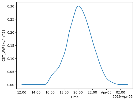
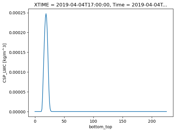
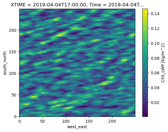
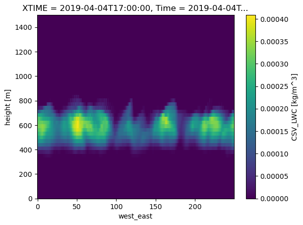
CSTare time series where all the spatial dimensions have been collapsed via averaging or vertical integration. An example isCST_LWPfor domain-average liquid water path.CSPare time series of profiles. The X-Y dimensions have been collapsed via averaging but vertical information is retained. The variable related toCST_LWPisCSP_LWCfor the domain-averaged liquid water content profile.CSSare time series of X-Y slices. Continuing on the theme of quantifying the condensate,CSS_LWPis the liquid water path with X-Y information retained.CSVare full-volume variables with X-Y-Z-T dimensions. A condensate example would beCSV_QRfor the rainwater mixing ratio. This is similar to theQRAINvariable output normally by WRF. However, the variables inwrfstatare averaged between output times, where as variables in thewrfoutfiles are instantaneous.
Plotting wrfstat data is straightforward since all output times from a run are included in one file.
# By default, xarray does not interpret the wrfout/wrfstat time information in a way that attaches
# it to each variable. Here is at trick to map the time held in XTIME with the Time coordinate
# associated with each variable.
ds_stat["Time"] = ds_stat["XTIME"]

# Now that we fixed the time coordinate, we can use xarray's plotting features to get time-labeled plots.

hour_to_plot = 17

# Time series:
ds_stat["CST_LWP"].plot()
plt.show()

# Profile at a selected time (plots sideways, though, since we are being lazy):
ds_stat["CSP_LWC"].sel(Time=f"{case_date:%Y-%m-%d} {hour_to_plot}:00").plot()
plt.show()

# X-Y slice for a selected time:
ds_stat["CSS_LWP"].sel(Time=f"{case_date:%Y-%m-%d} {hour_to_plot}:00").plot()
plt.show()

# A vertical slice from the volume at a selected time:
# We'll assign the vertical coordinate values for this one and hide the cloud-free upper atmosphere.
plot_data = ds_stat["CSV_LWC"].assign_coords(height=(ds_stat["CSP_Z"]))
plot_data.sel(Time=f"{case_date:%Y-%m-%d} {hour_to_plot}:00", south_north=1).plot(y="height", ylim=[0, 1500])
plt.show()
This is a good point to check out part 2 of the LASSO-ShCu tutorial, lasso-shcu_part2.ipynb. That shows how to do a 3-D isosurface plot of the LWC data. We isolate that in a separate notebook since the resulting file gets large and can cause rendring issues in some situations. Come back and continue here after looking at the part2 notebook.
In addition to the wrfstat file, the sgplassodiagraw dataset includes the instantaneous wrfout files, which contain one output time per wrfout. These files are essentially traditional WRF model output and can be read using one the WRF tools that exist in the wild such as xWRF or wrf-python. One can also hand-code the data parsing based on the level of detail needed for a particular application. This can be faster than using the more all-encompasing tools. See the xWRF tutorial for an example of using xWRF.
# Open a wrfout time series using a manual approach...

case_date = datetime(2019, 4, 4)
sim_id = 4

# Note the extra details required by open_mfdataset to connect the files together in time.
ds_wrf = xr.open_mfdataset(f"{path_shcu_root}/{case_date:%Y%m%d}/sim{sim_id:04d}/raw_model/wrfout_d01_*.nc",
                           combine="nested", concat_dim="Time")

ds_wrf["Time"] = ds_wrf["XTIME"]  # Fix the time coordinate like we did for the wrfstat file
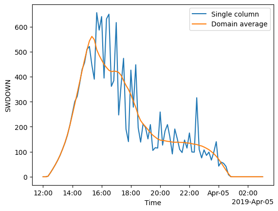
Let’s plot a time series of downwelling shortwave radiation.
Since all columns are statistically identical in this idealized model configuration, let’s plot the corner column and compare to a domain average.
fig, ax = plt.subplots(ncols=1)

ds_wrf["SWDOWN"].isel(west_east=0, south_north=0).plot(ax=ax, label="Single column")
ds_wrf["SWDOWN"].mean(dim=["west_east", "south_north"]).plot(ax=ax, label="Domain average")
ax.legend()

plt.show()
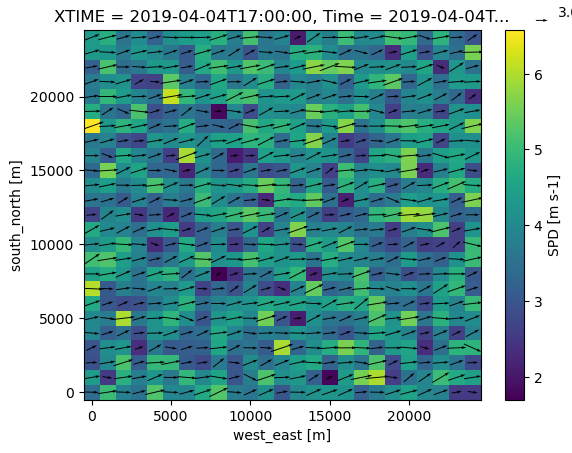
WRF uses an Arakawa C grid, which means the winds and height information are on cell edges, while the rest of the information is stored on the cell centers. Manually destaggering variables is where the approach of hand-coding the WRF processing becomes a bit annoying. Here is a quick example for the winds. U and V wind components are staggered in the X and Y directions, respectively. The height information is staggered in the vertical, but we will not deal with that in this notebook.
# Plot wind vectors at a selected level to demonstrate how to destagger the wind components to cell-center values with xarray...

plot_level = 12  # index of level to plot
skip_xy = 10  # Sampling interval for the vector thinning

nt, nz, ny, nx = ds_wrf["T"].shape

# We need to:
# 1) destagger to cell centers
# 2) rename the staggered dimension back to the non-staggered name to avoid dimension conflicts
# 3) (re)name the unstaggered wind for convenience
# Then, we are able to put these new DataArrays back into the ds_wrf Dataset.

ds_wrf["UA"] = 0.5*( ds_wrf["U"].isel(west_east_stag=slice(0, nx)) +
                    ds_wrf["U"].shift(west_east_stag=-1).isel(west_east_stag=slice(0, nx)) ).\
                    rename("UA").rename(west_east_stag="west_east")
ds_wrf["VA"] = 0.5*( ds_wrf["V"].isel(south_north_stag=slice(0, ny)) +
                    ds_wrf["V"].shift(south_north_stag=-1).isel(south_north_stag=slice(0, ny)) ).\
                    rename("VA").rename(south_north_stag="south_north")
ds_wrf["SPD"] = np.sqrt(ds_wrf["UA"]**2 + ds_wrf["VA"]**2).rename("wind speed").\
                    assign_attrs(units="m s-1", description="wind speed")

# Now, we can proceed to more plotting-specific data manipulation. We need to
# add spatial variables for the idealized domain (since XLAT and XLONG are
# constant in the file). This is needed by the xarray quiver routine.
# Then, thin the grid to reduce the number of arrrows.
ds_wrf["west_east"] = xr.DataArray(data=np.arange(nx)*ds_wrf.attrs["DX"], dims="west_east", name="west_east", attrs={"units": "m"})
ds_wrf["south_north"] = xr.DataArray(data=np.arange(ny)*ds_wrf.attrs["DX"], dims="south_north", name="south_north", attrs={"units": "m"})

ds_wrf_thinned = ds_wrf.\
    isel(west_east=slice(0, nx, skip_xy), south_north=slice(0, ny, skip_xy), bottom_top=plot_level).\
    sel(Time=f"{case_date:%Y-%m-%d} {hour_to_plot}:00")

fig, ax = plt.subplots(ncols=1)
ds_wrf_thinned["SPD"].plot(ax=ax, x="west_east", y="south_north")
ds_wrf_thinned.plot.quiver(ax=ax, x="west_east", y="south_north", u="UA", v="VA",
                           scale=100)
plt.show()
Next, let’s reproduce the above plot using xWRF to see how this is simpler. After opening the wrfout files with xWRF, note the extra variables added at the end of the variable list for wind_east and wind_north. These are the destaggered winds rotated to earth-relative directions. The rotation matters for map projections, but not for idealized runs like we have here. The other thing to note is that the west_east, south_north, and bottom_top coordinates are replaced by x, y, and z with proper units.
# Option 2 using xWRF...
# NOTE: requires xWRF >=0.0.4 to handle the idealized wrfout file from LASSO-ShCu

# Note the special arguments sent to open_mfdataset to piece together the files along the time dimension.
# Then, there is the extra xwrf postprocessing command on the end to destagger and set up coordinates.
ds_xwrf = xr.open_mfdataset(f"{path_shcu_root}/{case_date:%Y%m%d}/sim{sim_id:04d}/raw_model/wrfout_d01_*.nc", combine="nested", concat_dim="Time").xwrf.postprocess()
ds_xwrf
<xarray.Dataset> Size: 255GB
Dimensions:                    (Time: 91, y: 250, x: 250, soil_layers_stag: 5,
                                z: 226, x_stag: 251, y_stag: 251, z_stag: 227,
                                force_layers: 751)
Coordinates: (12/15)
    XLAT                       (y, x) float32 250kB dask.array<chunksize=(125, 125), meta=np.ndarray>
    XLONG                      (y, x) float32 250kB dask.array<chunksize=(125, 125), meta=np.ndarray>
    XTIME                      (Time) datetime64[ns] 728B dask.array<chunksize=(6,), meta=np.ndarray>
    XLAT_U                     (y, x_stag) float32 251kB dask.array<chunksize=(125, 126), meta=np.ndarray>
    XLONG_U                    (y, x_stag) float32 251kB dask.array<chunksize=(125, 126), meta=np.ndarray>
    XLAT_V                     (y_stag, x) float32 251kB dask.array<chunksize=(126, 125), meta=np.ndarray>
    ...                         ...
  * z_stag                     (z_stag) float32 908B 1.0 0.9959 ... 0.002178 0.0
  * Time                       (Time) datetime64[ns] 728B 2019-04-04T12:00:00...
  * x_stag                     (x_stag) float64 2kB -1.25e+04 ... 1.25e+04
  * x                          (x) float64 2kB -1.245e+04 ... 1.245e+04
  * y_stag                     (y_stag) float64 2kB -1.25e+04 ... 1.25e+04
  * y                          (y) float64 2kB -1.245e+04 ... 1.245e+04
Dimensions without coordinates: soil_layers_stag, force_layers
Data variables: (12/251)
    Times                      (Time) |S19 2kB dask.array<chunksize=(1,), meta=np.ndarray>
    LU_INDEX                   (Time, y, x) float32 23MB dask.array<chunksize=(1, 125, 125), meta=np.ndarray>
    ZS                         (Time, soil_layers_stag) float32 2kB dask.array<chunksize=(1, 5), meta=np.ndarray>
    DZS                        (Time, soil_layers_stag) float32 2kB dask.array<chunksize=(1, 5), meta=np.ndarray>
    VAR_SSO                    (Time, y, x) float32 23MB dask.array<chunksize=(1, 125, 125), meta=np.ndarray>
    U                          (Time, z, y, x_stag) float32 5GB dask.array<chunksize=(1, 226, 125, 126), meta=np.ndarray>
    ...                         ...
    geopotential               (Time, z_stag, y, x) float32 5GB dask.array<chunksize=(1, 227, 125, 125), meta=np.ndarray>
    geopotential_height        (Time, z_stag, y, x) float32 5GB dask.array<chunksize=(1, 227, 125, 125), meta=np.ndarray>
    wind_east                  (Time, z, y, x) float32 5GB dask.array<chunksize=(1, 226, 125, 125), meta=np.ndarray>
    wind_north                 (Time, z, y, x) float32 5GB dask.array<chunksize=(1, 226, 125, 125), meta=np.ndarray>
    wind_east_10               (Time, y, x) float32 23MB dask.array<chunksize=(1, 125, 125), meta=np.ndarray>
    wind_north_10              (Time, y, x) float32 23MB dask.array<chunksize=(1, 125, 125), meta=np.ndarray>
Attributes: (12/142)
    TITLE:                                  OUTPUT FROM WRF V3.8.1 MODEL
    START_DATE:                            2019-04-04_12:00:00
    SIMULATION_START_DATE:                 2019-04-04_12:00:00
    WEST-EAST_GRID_DIMENSION:              251
    SOUTH-NORTH_GRID_DIMENSION:            251
    BOTTOM-TOP_GRID_DIMENSION:             227
    ...                                    ...
    config_aerosol:                        NA
    config_forecast_time:                  15.0 h
    config_boundary_method:                Periodic
    config_microphysics:                   Thompson (mp_physics=8)
    config_nickname:                       runlas20190404v1addhm
simulation_origin_host: cumulus-login2.ccs.ornl.gov- Time: 91
- y: 250
- x: 250
- soil_layers_stag: 5
- z: 226
- x_stag: 251
- y_stag: 251
- z_stag: 227
- force_layers: 751
- XLAT(y, x)float32dask.array<chunksize=(125, 125), meta=np.ndarray>
- FieldType :
- 104
- MemoryOrder :
- XY
- description :
- LATITUDE, SOUTH IS NEGATIVE
- units :
- degree_north
- stagger :
Array Chunk Bytes 244.14 kiB 61.04 kiB Shape (250, 250) (125, 125) Dask graph 4 chunks in 34 graph layers Data type float32 numpy.ndarray - XLONG(y, x)float32dask.array<chunksize=(125, 125), meta=np.ndarray>
- FieldType :
- 104
- MemoryOrder :
- XY
- description :
- LONGITUDE, WEST IS NEGATIVE
- units :
- degree_east
- stagger :
Array Chunk Bytes 244.14 kiB 61.04 kiB Shape (250, 250) (125, 125) Dask graph 4 chunks in 34 graph layers Data type float32 numpy.ndarray - XTIME(Time)datetime64[ns]dask.array<chunksize=(6,), meta=np.ndarray>
- FieldType :
- 104
- MemoryOrder :
- 0
- description :
- minutes since 2019-04-04 12:00:00
- stagger :
Array Chunk Bytes 728 B 48 B Shape (91,) (6,) Dask graph 16 chunks in 33 graph layers Data type datetime64[ns] numpy.ndarray - XLAT_U(y, x_stag)float32dask.array<chunksize=(125, 126), meta=np.ndarray>
- FieldType :
- 104
- MemoryOrder :
- XY
- description :
- LATITUDE, SOUTH IS NEGATIVE
- units :
- degree_north
- stagger :
- X
Array Chunk Bytes 245.12 kiB 61.52 kiB Shape (250, 251) (125, 126) Dask graph 4 chunks in 34 graph layers Data type float32 numpy.ndarray - XLONG_U(y, x_stag)float32dask.array<chunksize=(125, 126), meta=np.ndarray>
- FieldType :
- 104
- MemoryOrder :
- XY
- description :
- LONGITUDE, WEST IS NEGATIVE
- units :
- degree_east
- stagger :
- X
Array Chunk Bytes 245.12 kiB 61.52 kiB Shape (250, 251) (125, 126) Dask graph 4 chunks in 34 graph layers Data type float32 numpy.ndarray - XLAT_V(y_stag, x)float32dask.array<chunksize=(126, 125), meta=np.ndarray>
- FieldType :
- 104
- MemoryOrder :
- XY
- description :
- LATITUDE, SOUTH IS NEGATIVE
- units :
- degree_north
- stagger :
- Y
Array Chunk Bytes 245.12 kiB 61.52 kiB Shape (251, 250) (126, 125) Dask graph 4 chunks in 34 graph layers Data type float32 numpy.ndarray - XLONG_V(y_stag, x)float32dask.array<chunksize=(126, 125), meta=np.ndarray>
- FieldType :
- 104
- MemoryOrder :
- XY
- description :
- LONGITUDE, WEST IS NEGATIVE
- units :
- degree_east
- stagger :
- Y
Array Chunk Bytes 245.12 kiB 61.52 kiB Shape (251, 250) (126, 125) Dask graph 4 chunks in 34 graph layers Data type float32 numpy.ndarray - CLAT(y, x)float32dask.array<chunksize=(125, 125), meta=np.ndarray>
- FieldType :
- 104
- MemoryOrder :
- XY
- description :
- COMPUTATIONAL GRID LATITUDE, SOUTH IS NEGATIVE
- units :
- degree_north
- stagger :
Array Chunk Bytes 244.14 kiB 61.04 kiB Shape (250, 250) (125, 125) Dask graph 4 chunks in 34 graph layers Data type float32 numpy.ndarray - z(z)float320.9979 0.9938 ... 0.005743 0.001089
- FieldType :
- 104
- MemoryOrder :
- Z
- description :
- eta values on half (mass) levels
- units :
- stagger :
- axis :
- Z
- standard_name :
- atmosphere_sigma_coordinate
array([0.997944, 0.993847, 0.989777, ..., 0.01304 , 0.005743, 0.001089], dtype=float32) - z_stag(z_stag)float321.0 0.9959 0.9918 ... 0.002178 0.0
- FieldType :
- 104
- MemoryOrder :
- Z
- description :
- eta values on full (w) levels
- units :
- stagger :
- Z
- axis :
- Z
- c_grid_axis_shift :
- 0.5
- standard_name :
- atmosphere_sigma_coordinate
array([1. , 0.995887, 0.991808, ..., 0.009308, 0.002178, 0. ], dtype=float32) - Time(Time)datetime64[ns]2019-04-04T12:00:00 ... 2019-04-...
- long_name :
- Time
- standard_name :
- time
array(['2019-04-04T12:00:00.000000000', '2019-04-04T12:10:00.000000000', '2019-04-04T12:20:00.000000000', '2019-04-04T12:30:00.000000000', '2019-04-04T12:40:00.000000000', '2019-04-04T12:50:00.000000000', '2019-04-04T13:00:00.000000000', '2019-04-04T13:10:00.000000000', '2019-04-04T13:20:00.000000000', '2019-04-04T13:30:00.000000000', '2019-04-04T13:40:00.000000000', '2019-04-04T13:50:00.000000000', '2019-04-04T14:00:00.000000000', '2019-04-04T14:10:00.000000000', '2019-04-04T14:20:00.000000000', '2019-04-04T14:30:00.000000000', '2019-04-04T14:40:00.000000000', '2019-04-04T14:50:00.000000000', '2019-04-04T15:00:00.000000000', '2019-04-04T15:10:00.000000000', '2019-04-04T15:20:00.000000000', '2019-04-04T15:30:00.000000000', '2019-04-04T15:40:00.000000000', '2019-04-04T15:50:00.000000000', '2019-04-04T16:00:00.000000000', '2019-04-04T16:10:00.000000000', '2019-04-04T16:20:00.000000000', '2019-04-04T16:30:00.000000000', '2019-04-04T16:40:00.000000000', '2019-04-04T16:50:00.000000000', '2019-04-04T17:00:00.000000000', '2019-04-04T17:10:00.000000000', '2019-04-04T17:20:00.000000000', '2019-04-04T17:30:00.000000000', '2019-04-04T17:40:00.000000000', '2019-04-04T17:50:00.000000000', '2019-04-04T18:00:00.000000000', '2019-04-04T18:10:00.000000000', '2019-04-04T18:20:00.000000000', '2019-04-04T18:30:00.000000000', '2019-04-04T18:40:00.000000000', '2019-04-04T18:50:00.000000000', '2019-04-04T19:00:00.000000000', '2019-04-04T19:10:00.000000000', '2019-04-04T19:20:00.000000000', '2019-04-04T19:30:00.000000000', '2019-04-04T19:40:00.000000000', '2019-04-04T19:50:00.000000000', '2019-04-04T20:00:00.000000000', '2019-04-04T20:10:00.000000000', '2019-04-04T20:20:00.000000000', '2019-04-04T20:30:00.000000000', '2019-04-04T20:40:00.000000000', '2019-04-04T20:50:00.000000000', '2019-04-04T21:00:00.000000000', '2019-04-04T21:10:00.000000000', '2019-04-04T21:20:00.000000000', '2019-04-04T21:30:00.000000000', '2019-04-04T21:40:00.000000000', '2019-04-04T21:50:00.000000000', '2019-04-04T22:00:00.000000000', '2019-04-04T22:10:00.000000000', '2019-04-04T22:20:00.000000000', '2019-04-04T22:30:00.000000000', '2019-04-04T22:40:00.000000000', '2019-04-04T22:50:00.000000000', '2019-04-04T23:00:00.000000000', '2019-04-04T23:10:00.000000000', '2019-04-04T23:20:00.000000000', '2019-04-04T23:30:00.000000000', '2019-04-04T23:40:00.000000000', '2019-04-04T23:50:00.000000000', '2019-04-05T00:00:00.000000000', '2019-04-05T00:10:00.000000000', '2019-04-05T00:20:00.000000000', '2019-04-05T00:30:00.000000000', '2019-04-05T00:40:00.000000000', '2019-04-05T00:50:00.000000000', '2019-04-05T01:00:00.000000000', '2019-04-05T01:10:00.000000000', '2019-04-05T01:20:00.000000000', '2019-04-05T01:30:00.000000000', '2019-04-05T01:40:00.000000000', '2019-04-05T01:50:00.000000000', '2019-04-05T02:00:00.000000000', '2019-04-05T02:10:00.000000000', '2019-04-05T02:20:00.000000000', '2019-04-05T02:30:00.000000000', '2019-04-05T02:40:00.000000000', '2019-04-05T02:50:00.000000000', '2019-04-05T03:00:00.000000000'], dtype='datetime64[ns]') - x_stag(x_stag)float64-1.25e+04 -1.24e+04 ... 1.25e+04
- units :
- m
- standard_name :
- projection_x_coordinate
- axis :
- X
- c_grid_axis_shift :
- 0.5
array([-12500., -12400., -12300., ..., 12300., 12400., 12500.])
- x(x)float64-1.245e+04 -1.235e+04 ... 1.245e+04
- units :
- m
- standard_name :
- projection_x_coordinate
- axis :
- X
array([-12450., -12350., -12250., ..., 12250., 12350., 12450.])
- y_stag(y_stag)float64-1.25e+04 -1.24e+04 ... 1.25e+04
- units :
- m
- standard_name :
- projection_y_coordinate
- axis :
- Y
- c_grid_axis_shift :
- 0.5
array([-12500., -12400., -12300., ..., 12300., 12400., 12500.])
- y(y)float64-1.245e+04 -1.235e+04 ... 1.245e+04
- units :
- m
- standard_name :
- projection_y_coordinate
- axis :
- Y
array([-12450., -12350., -12250., ..., 12250., 12350., 12450.])
- Times(Time)|S19dask.array<chunksize=(1,), meta=np.ndarray>
Array Chunk Bytes 1.69 kiB 19 B Shape (91,) (1,) Dask graph 91 chunks in 33 graph layers Data type |S19 numpy.ndarray - LU_INDEX(Time, y, x)float32dask.array<chunksize=(1, 125, 125), meta=np.ndarray>
- FieldType :
- 104
- MemoryOrder :
- XY
- description :
- LAND USE CATEGORY
- units :
- stagger :
Array Chunk Bytes 21.70 MiB 61.04 kiB Shape (91, 250, 250) (1, 125, 125) Dask graph 364 chunks in 33 graph layers Data type float32 numpy.ndarray - ZS(Time, soil_layers_stag)float32dask.array<chunksize=(1, 5), meta=np.ndarray>
- FieldType :
- 104
- MemoryOrder :
- Z
- description :
- DEPTHS OF CENTERS OF SOIL LAYERS
- units :
- m
- stagger :
- Z
Array Chunk Bytes 1.78 kiB 20 B Shape (91, 5) (1, 5) Dask graph 91 chunks in 33 graph layers Data type float32 numpy.ndarray - DZS(Time, soil_layers_stag)float32dask.array<chunksize=(1, 5), meta=np.ndarray>
- FieldType :
- 104
- MemoryOrder :
- Z
- description :
- THICKNESSES OF SOIL LAYERS
- units :
- m
- stagger :
- Z
Array Chunk Bytes 1.78 kiB 20 B Shape (91, 5) (1, 5) Dask graph 91 chunks in 33 graph layers Data type float32 numpy.ndarray - VAR_SSO(Time, y, x)float32dask.array<chunksize=(1, 125, 125), meta=np.ndarray>
- FieldType :
- 104
- MemoryOrder :
- XY
- description :
- Variance of Subgrid Scale Orography MSL
- units :
- m2
- stagger :
Array Chunk Bytes 21.70 MiB 61.04 kiB Shape (91, 250, 250) (1, 125, 125) Dask graph 364 chunks in 33 graph layers Data type float32 numpy.ndarray - U(Time, z, y, x_stag)float32dask.array<chunksize=(1, 226, 125, 126), meta=np.ndarray>
- FieldType :
- 104
- MemoryOrder :
- XYZ
- description :
- x-wind component
- units :
- m s-1
- stagger :
- X
- standard_name :
- x_wind
Array Chunk Bytes 4.81 GiB 13.58 MiB Shape (91, 226, 250, 251) (1, 226, 125, 126) Dask graph 364 chunks in 33 graph layers Data type float32 numpy.ndarray - V(Time, z, y_stag, x)float32dask.array<chunksize=(1, 226, 126, 125), meta=np.ndarray>
- FieldType :
- 104
- MemoryOrder :
- XYZ
- description :
- y-wind component
- units :
- m s-1
- stagger :
- Y
- standard_name :
- y_wind
Array Chunk Bytes 4.81 GiB 13.58 MiB Shape (91, 226, 251, 250) (1, 226, 126, 125) Dask graph 364 chunks in 33 graph layers Data type float32 numpy.ndarray - W(Time, z_stag, y, x)float32dask.array<chunksize=(1, 227, 125, 125), meta=np.ndarray>
- FieldType :
- 104
- MemoryOrder :
- XYZ
- description :
- z-wind component
- units :
- m s-1
- stagger :
- Z
- standard_name :
- upward_air_velocity
Array Chunk Bytes 4.81 GiB 13.53 MiB Shape (91, 227, 250, 250) (1, 227, 125, 125) Dask graph 364 chunks in 33 graph layers Data type float32 numpy.ndarray - HFX_FORCE(Time)float32dask.array<chunksize=(6,), meta=np.ndarray>
- FieldType :
- 104
- MemoryOrder :
- 0
- description :
- SCM ideal surface sensible heat flux
- units :
- W m-2
- stagger :
Array Chunk Bytes 364 B 24 B Shape (91,) (6,) Dask graph 16 chunks in 33 graph layers Data type float32 numpy.ndarray - LH_FORCE(Time)float32dask.array<chunksize=(6,), meta=np.ndarray>
- FieldType :
- 104
- MemoryOrder :
- 0
- description :
- SCM ideal surface latent heat flux
- units :
- W m-2
- stagger :
Array Chunk Bytes 364 B 24 B Shape (91,) (6,) Dask graph 16 chunks in 33 graph layers Data type float32 numpy.ndarray - TSK_FORCE(Time)float32dask.array<chunksize=(6,), meta=np.ndarray>
- FieldType :
- 104
- MemoryOrder :
- 0
- description :
- SCM ideal surface skin temperature
- units :
- W m-2
- stagger :
Array Chunk Bytes 364 B 24 B Shape (91,) (6,) Dask graph 16 chunks in 33 graph layers Data type float32 numpy.ndarray - HFX_FORCE_TEND(Time)float32dask.array<chunksize=(6,), meta=np.ndarray>
- FieldType :
- 104
- MemoryOrder :
- 0
- description :
- SCM ideal surface sensible heat flux tendency
- units :
- W m-2 s-1
- stagger :
Array Chunk Bytes 364 B 24 B Shape (91,) (6,) Dask graph 16 chunks in 33 graph layers Data type float32 numpy.ndarray - LH_FORCE_TEND(Time)float32dask.array<chunksize=(6,), meta=np.ndarray>
- FieldType :
- 104
- MemoryOrder :
- 0
- description :
- SCM ideal surface latent heat flux tendency
- units :
- W m-2 s-1
- stagger :
Array Chunk Bytes 364 B 24 B Shape (91,) (6,) Dask graph 16 chunks in 33 graph layers Data type float32 numpy.ndarray - TSK_FORCE_TEND(Time)float32dask.array<chunksize=(6,), meta=np.ndarray>
- FieldType :
- 104
- MemoryOrder :
- 0
- description :
- SCM ideal surface skin temperature tendency
- units :
- W m-2 s-1
- stagger :
Array Chunk Bytes 364 B 24 B Shape (91,) (6,) Dask graph 16 chunks in 33 graph layers Data type float32 numpy.ndarray - MU(Time, y, x)float32dask.array<chunksize=(1, 125, 125), meta=np.ndarray>
- FieldType :
- 104
- MemoryOrder :
- XY
- description :
- perturbation dry air mass in column
- units :
- Pa
- stagger :
Array Chunk Bytes 21.70 MiB 61.04 kiB Shape (91, 250, 250) (1, 125, 125) Dask graph 364 chunks in 33 graph layers Data type float32 numpy.ndarray - MUB(Time, y, x)float32dask.array<chunksize=(1, 125, 125), meta=np.ndarray>
- FieldType :
- 104
- MemoryOrder :
- XY
- description :
- base state dry air mass in column
- units :
- Pa
- stagger :
Array Chunk Bytes 21.70 MiB 61.04 kiB Shape (91, 250, 250) (1, 125, 125) Dask graph 364 chunks in 33 graph layers Data type float32 numpy.ndarray - NEST_POS(Time, y, x)float32dask.array<chunksize=(1, 125, 125), meta=np.ndarray>
- FieldType :
- 104
- MemoryOrder :
- XY
- description :
- -
- stagger :
Array Chunk Bytes 21.70 MiB 61.04 kiB Shape (91, 250, 250) (1, 125, 125) Dask graph 364 chunks in 33 graph layers Data type float32 numpy.ndarray - TKE(Time, z, y, x)float32dask.array<chunksize=(1, 226, 125, 125), meta=np.ndarray>
- FieldType :
- 104
- MemoryOrder :
- XYZ
- description :
- TURBULENCE KINETIC ENERGY
- units :
- m2 s-2
- stagger :
Array Chunk Bytes 4.79 GiB 13.47 MiB Shape (91, 226, 250, 250) (1, 226, 125, 125) Dask graph 364 chunks in 33 graph layers Data type float32 numpy.ndarray - ALT(Time, z, y, x)float32dask.array<chunksize=(1, 226, 125, 125), meta=np.ndarray>
- FieldType :
- 104
- MemoryOrder :
- XYZ
- description :
- inverse density
- units :
- m3 kg-1
- stagger :
Array Chunk Bytes 4.79 GiB 13.47 MiB Shape (91, 226, 250, 250) (1, 226, 125, 125) Dask graph 364 chunks in 33 graph layers Data type float32 numpy.ndarray - FNM(Time, z)float32dask.array<chunksize=(1, 226), meta=np.ndarray>
- FieldType :
- 104
- MemoryOrder :
- Z
- description :
- upper weight for vertical stretching
- units :
- stagger :
Array Chunk Bytes 80.34 kiB 904 B Shape (91, 226) (1, 226) Dask graph 91 chunks in 33 graph layers Data type float32 numpy.ndarray - FNP(Time, z)float32dask.array<chunksize=(1, 226), meta=np.ndarray>
- FieldType :
- 104
- MemoryOrder :
- Z
- description :
- lower weight for vertical stretching
- units :
- stagger :
Array Chunk Bytes 80.34 kiB 904 B Shape (91, 226) (1, 226) Dask graph 91 chunks in 33 graph layers Data type float32 numpy.ndarray - RDNW(Time, z)float32dask.array<chunksize=(1, 226), meta=np.ndarray>
- FieldType :
- 104
- MemoryOrder :
- Z
- description :
- inverse d(eta) values between full (w) levels
- units :
- stagger :
Array Chunk Bytes 80.34 kiB 904 B Shape (91, 226) (1, 226) Dask graph 91 chunks in 33 graph layers Data type float32 numpy.ndarray - RDN(Time, z)float32dask.array<chunksize=(1, 226), meta=np.ndarray>
- FieldType :
- 104
- MemoryOrder :
- Z
- description :
- inverse d(eta) values between half (mass) levels
- units :
- stagger :
Array Chunk Bytes 80.34 kiB 904 B Shape (91, 226) (1, 226) Dask graph 91 chunks in 33 graph layers Data type float32 numpy.ndarray - DNW(Time, z)float32dask.array<chunksize=(1, 226), meta=np.ndarray>
- FieldType :
- 104
- MemoryOrder :
- Z
- description :
- d(eta) values between full (w) levels
- units :
- stagger :
Array Chunk Bytes 80.34 kiB 904 B Shape (91, 226) (1, 226) Dask graph 91 chunks in 33 graph layers Data type float32 numpy.ndarray - DN(Time, z)float32dask.array<chunksize=(1, 226), meta=np.ndarray>
- FieldType :
- 104
- MemoryOrder :
- Z
- description :
- d(eta) values between half (mass) levels
- units :
- stagger :
Array Chunk Bytes 80.34 kiB 904 B Shape (91, 226) (1, 226) Dask graph 91 chunks in 33 graph layers Data type float32 numpy.ndarray - CFN(Time)float32dask.array<chunksize=(6,), meta=np.ndarray>
- FieldType :
- 104
- MemoryOrder :
- 0
- description :
- extrapolation constant
- units :
- stagger :
Array Chunk Bytes 364 B 24 B Shape (91,) (6,) Dask graph 16 chunks in 33 graph layers Data type float32 numpy.ndarray - CFN1(Time)float32dask.array<chunksize=(6,), meta=np.ndarray>
- FieldType :
- 104
- MemoryOrder :
- 0
- description :
- extrapolation constant
- units :
- stagger :
Array Chunk Bytes 364 B 24 B Shape (91,) (6,) Dask graph 16 chunks in 33 graph layers Data type float32 numpy.ndarray - THIS_IS_AN_IDEAL_RUN(Time)int32dask.array<chunksize=(6,), meta=np.ndarray>
- FieldType :
- 106
- MemoryOrder :
- 0
- description :
- T/F flag: this is an ARW ideal simulation
- stagger :
Array Chunk Bytes 364 B 24 B Shape (91,) (6,) Dask graph 16 chunks in 33 graph layers Data type int32 numpy.ndarray - P_HYD(Time, z, y, x)float32dask.array<chunksize=(1, 226, 125, 125), meta=np.ndarray>
- FieldType :
- 104
- MemoryOrder :
- XYZ
- description :
- hydrostatic pressure
- units :
- Pa
- stagger :
Array Chunk Bytes 4.79 GiB 13.47 MiB Shape (91, 226, 250, 250) (1, 226, 125, 125) Dask graph 364 chunks in 33 graph layers Data type float32 numpy.ndarray - Q2(Time, y, x)float32dask.array<chunksize=(1, 125, 125), meta=np.ndarray>
- FieldType :
- 104
- MemoryOrder :
- XY
- description :
- QV at 2 M
- units :
- kg kg-1
- stagger :
- standard_name :
- humidity_mixing_ratio
- long_name :
- humidity_mixing_ratio_at_2m_agl
Array Chunk Bytes 21.70 MiB 61.04 kiB Shape (91, 250, 250) (1, 125, 125) Dask graph 364 chunks in 33 graph layers Data type float32 numpy.ndarray - T2(Time, y, x)float32dask.array<chunksize=(1, 125, 125), meta=np.ndarray>
- FieldType :
- 104
- MemoryOrder :
- XY
- description :
- TEMP at 2 M
- units :
- K
- stagger :
- standard_name :
- air_temperature
- long_name :
- air_temperature_at_2m_agl
Array Chunk Bytes 21.70 MiB 61.04 kiB Shape (91, 250, 250) (1, 125, 125) Dask graph 364 chunks in 33 graph layers Data type float32 numpy.ndarray - TH2(Time, y, x)float32dask.array<chunksize=(1, 125, 125), meta=np.ndarray>
- FieldType :
- 104
- MemoryOrder :
- XY
- description :
- POT TEMP at 2 M
- units :
- K
- stagger :
- standard_name :
- air_potential_temperature
- long_name :
- air_potential_temperature_at_2m_agl
Array Chunk Bytes 21.70 MiB 61.04 kiB Shape (91, 250, 250) (1, 125, 125) Dask graph 364 chunks in 33 graph layers Data type float32 numpy.ndarray - PSFC(Time, y, x)float32dask.array<chunksize=(1, 125, 125), meta=np.ndarray>
- FieldType :
- 104
- MemoryOrder :
- XY
- description :
- SFC PRESSURE
- units :
- Pa
- stagger :
- standard_name :
- air_pressure
- long_name :
- air_pressure_at_surface
Array Chunk Bytes 21.70 MiB 61.04 kiB Shape (91, 250, 250) (1, 125, 125) Dask graph 364 chunks in 33 graph layers Data type float32 numpy.ndarray - U10(Time, y, x)float32dask.array<chunksize=(1, 125, 125), meta=np.ndarray>
- FieldType :
- 104
- MemoryOrder :
- XY
- description :
- U at 10 M
- units :
- m s-1
- stagger :
- standard_name :
- x_wind
- long_name :
- x_wind_at_10m_agl
Array Chunk Bytes 21.70 MiB 61.04 kiB Shape (91, 250, 250) (1, 125, 125) Dask graph 364 chunks in 33 graph layers Data type float32 numpy.ndarray - V10(Time, y, x)float32dask.array<chunksize=(1, 125, 125), meta=np.ndarray>
- FieldType :
- 104
- MemoryOrder :
- XY
- description :
- V at 10 M
- units :
- m s-1
- stagger :
- standard_name :
- y_wind
- long_name :
- y_wind_at_10m_agl
Array Chunk Bytes 21.70 MiB 61.04 kiB Shape (91, 250, 250) (1, 125, 125) Dask graph 364 chunks in 33 graph layers Data type float32 numpy.ndarray - RDX(Time)float32dask.array<chunksize=(6,), meta=np.ndarray>
- FieldType :
- 104
- MemoryOrder :
- 0
- description :
- INVERSE X GRID LENGTH
- units :
- stagger :
Array Chunk Bytes 364 B 24 B Shape (91,) (6,) Dask graph 16 chunks in 33 graph layers Data type float32 numpy.ndarray - RDY(Time)float32dask.array<chunksize=(6,), meta=np.ndarray>
- FieldType :
- 104
- MemoryOrder :
- 0
- description :
- INVERSE Y GRID LENGTH
- units :
- stagger :
Array Chunk Bytes 364 B 24 B Shape (91,) (6,) Dask graph 16 chunks in 33 graph layers Data type float32 numpy.ndarray - RESM(Time)float32dask.array<chunksize=(6,), meta=np.ndarray>
- FieldType :
- 104
- MemoryOrder :
- 0
- description :
- TIME WEIGHT CONSTANT FOR SMALL STEPS
- units :
- stagger :
Array Chunk Bytes 364 B 24 B Shape (91,) (6,) Dask graph 16 chunks in 33 graph layers Data type float32 numpy.ndarray - ZETATOP(Time)float32dask.array<chunksize=(6,), meta=np.ndarray>
- FieldType :
- 104
- MemoryOrder :
- 0
- description :
- ZETA AT MODEL TOP
- units :
- stagger :
Array Chunk Bytes 364 B 24 B Shape (91,) (6,) Dask graph 16 chunks in 33 graph layers Data type float32 numpy.ndarray - CF1(Time)float32dask.array<chunksize=(6,), meta=np.ndarray>
- FieldType :
- 104
- MemoryOrder :
- 0
- description :
- 2nd order extrapolation constant
- units :
- stagger :
Array Chunk Bytes 364 B 24 B Shape (91,) (6,) Dask graph 16 chunks in 33 graph layers Data type float32 numpy.ndarray - CF2(Time)float32dask.array<chunksize=(6,), meta=np.ndarray>
- FieldType :
- 104
- MemoryOrder :
- 0
- description :
- 2nd order extrapolation constant
- units :
- stagger :
Array Chunk Bytes 364 B 24 B Shape (91,) (6,) Dask graph 16 chunks in 33 graph layers Data type float32 numpy.ndarray - CF3(Time)float32dask.array<chunksize=(6,), meta=np.ndarray>
- FieldType :
- 104
- MemoryOrder :
- 0
- description :
- 2nd order extrapolation constant
- units :
- stagger :
Array Chunk Bytes 364 B 24 B Shape (91,) (6,) Dask graph 16 chunks in 33 graph layers Data type float32 numpy.ndarray - ITIMESTEP(Time)int32dask.array<chunksize=(6,), meta=np.ndarray>
- FieldType :
- 106
- MemoryOrder :
- 0
- description :
- units :
- stagger :
Array Chunk Bytes 364 B 24 B Shape (91,) (6,) Dask graph 16 chunks in 33 graph layers Data type int32 numpy.ndarray - QVAPOR(Time, z, y, x)float32dask.array<chunksize=(1, 226, 125, 125), meta=np.ndarray>
- FieldType :
- 104
- MemoryOrder :
- XYZ
- description :
- Water vapor mixing ratio
- units :
- kg kg-1
- stagger :
- standard_name :
- humidity_mixing_ratio
Array Chunk Bytes 4.79 GiB 13.47 MiB Shape (91, 226, 250, 250) (1, 226, 125, 125) Dask graph 364 chunks in 33 graph layers Data type float32 numpy.ndarray - QCLOUD(Time, z, y, x)float32dask.array<chunksize=(1, 226, 125, 125), meta=np.ndarray>
- FieldType :
- 104
- MemoryOrder :
- XYZ
- description :
- Cloud water mixing ratio
- units :
- kg kg-1
- stagger :
Array Chunk Bytes 4.79 GiB 13.47 MiB Shape (91, 226, 250, 250) (1, 226, 125, 125) Dask graph 364 chunks in 33 graph layers Data type float32 numpy.ndarray - QRAIN(Time, z, y, x)float32dask.array<chunksize=(1, 226, 125, 125), meta=np.ndarray>
- FieldType :
- 104
- MemoryOrder :
- XYZ
- description :
- Rain water mixing ratio
- units :
- kg kg-1
- stagger :
Array Chunk Bytes 4.79 GiB 13.47 MiB Shape (91, 226, 250, 250) (1, 226, 125, 125) Dask graph 364 chunks in 33 graph layers Data type float32 numpy.ndarray - QICE(Time, z, y, x)float32dask.array<chunksize=(1, 226, 125, 125), meta=np.ndarray>
- FieldType :
- 104
- MemoryOrder :
- XYZ
- description :
- Ice mixing ratio
- units :
- kg kg-1
- stagger :
Array Chunk Bytes 4.79 GiB 13.47 MiB Shape (91, 226, 250, 250) (1, 226, 125, 125) Dask graph 364 chunks in 33 graph layers Data type float32 numpy.ndarray - QSNOW(Time, z, y, x)float32dask.array<chunksize=(1, 226, 125, 125), meta=np.ndarray>
- FieldType :
- 104
- MemoryOrder :
- XYZ
- description :
- Snow mixing ratio
- units :
- kg kg-1
- stagger :
Array Chunk Bytes 4.79 GiB 13.47 MiB Shape (91, 226, 250, 250) (1, 226, 125, 125) Dask graph 364 chunks in 33 graph layers Data type float32 numpy.ndarray - QGRAUP(Time, z, y, x)float32dask.array<chunksize=(1, 226, 125, 125), meta=np.ndarray>
- FieldType :
- 104
- MemoryOrder :
- XYZ
- description :
- Graupel mixing ratio
- units :
- kg kg-1
- stagger :
Array Chunk Bytes 4.79 GiB 13.47 MiB Shape (91, 226, 250, 250) (1, 226, 125, 125) Dask graph 364 chunks in 33 graph layers Data type float32 numpy.ndarray - QNICE(Time, z, y, x)float32dask.array<chunksize=(1, 226, 125, 125), meta=np.ndarray>
- FieldType :
- 104
- MemoryOrder :
- XYZ
- description :
- Ice Number concentration
- units :
- kg-1
- stagger :
Array Chunk Bytes 4.79 GiB 13.47 MiB Shape (91, 226, 250, 250) (1, 226, 125, 125) Dask graph 364 chunks in 33 graph layers Data type float32 numpy.ndarray - QNRAIN(Time, z, y, x)float32dask.array<chunksize=(1, 226, 125, 125), meta=np.ndarray>
- FieldType :
- 104
- MemoryOrder :
- XYZ
- description :
- Rain Number concentration
- units :
- kg-1
- stagger :
Array Chunk Bytes 4.79 GiB 13.47 MiB Shape (91, 226, 250, 250) (1, 226, 125, 125) Dask graph 364 chunks in 33 graph layers Data type float32 numpy.ndarray - SHDMAX(Time, y, x)float32dask.array<chunksize=(1, 125, 125), meta=np.ndarray>
- FieldType :
- 104
- MemoryOrder :
- XY
- description :
- ANNUAL MAX VEG FRACTION
- units :
- stagger :
Array Chunk Bytes 21.70 MiB 61.04 kiB Shape (91, 250, 250) (1, 125, 125) Dask graph 364 chunks in 33 graph layers Data type float32 numpy.ndarray - SHDMIN(Time, y, x)float32dask.array<chunksize=(1, 125, 125), meta=np.ndarray>
- FieldType :
- 104
- MemoryOrder :
- XY
- description :
- ANNUAL MIN VEG FRACTION
- units :
- stagger :
Array Chunk Bytes 21.70 MiB 61.04 kiB Shape (91, 250, 250) (1, 125, 125) Dask graph 364 chunks in 33 graph layers Data type float32 numpy.ndarray - SNOALB(Time, y, x)float32dask.array<chunksize=(1, 125, 125), meta=np.ndarray>
- FieldType :
- 104
- MemoryOrder :
- XY
- description :
- ANNUAL MAX SNOW ALBEDO IN FRACTION
- units :
- stagger :
Array Chunk Bytes 21.70 MiB 61.04 kiB Shape (91, 250, 250) (1, 125, 125) Dask graph 364 chunks in 33 graph layers Data type float32 numpy.ndarray - TSLB(Time, soil_layers_stag, y, x)float32dask.array<chunksize=(1, 5, 125, 125), meta=np.ndarray>
- FieldType :
- 104
- MemoryOrder :
- XYZ
- description :
- SOIL TEMPERATURE
- units :
- K
- stagger :
- Z
Array Chunk Bytes 108.48 MiB 305.18 kiB Shape (91, 5, 250, 250) (1, 5, 125, 125) Dask graph 364 chunks in 33 graph layers Data type float32 numpy.ndarray - SMOIS(Time, soil_layers_stag, y, x)float32dask.array<chunksize=(1, 5, 125, 125), meta=np.ndarray>
- FieldType :
- 104
- MemoryOrder :
- XYZ
- description :
- SOIL MOISTURE
- units :
- m3 m-3
- stagger :
- Z
Array Chunk Bytes 108.48 MiB 305.18 kiB Shape (91, 5, 250, 250) (1, 5, 125, 125) Dask graph 364 chunks in 33 graph layers Data type float32 numpy.ndarray - SH2O(Time, soil_layers_stag, y, x)float32dask.array<chunksize=(1, 5, 125, 125), meta=np.ndarray>
- FieldType :
- 104
- MemoryOrder :
- XYZ
- description :
- SOIL LIQUID WATER
- units :
- m3 m-3
- stagger :
- Z
Array Chunk Bytes 108.48 MiB 305.18 kiB Shape (91, 5, 250, 250) (1, 5, 125, 125) Dask graph 364 chunks in 33 graph layers Data type float32 numpy.ndarray - SEAICE(Time, y, x)float32dask.array<chunksize=(1, 125, 125), meta=np.ndarray>
- FieldType :
- 104
- MemoryOrder :
- XY
- description :
- SEA ICE FLAG
- units :
- stagger :
Array Chunk Bytes 21.70 MiB 61.04 kiB Shape (91, 250, 250) (1, 125, 125) Dask graph 364 chunks in 33 graph layers Data type float32 numpy.ndarray - XICEM(Time, y, x)float32dask.array<chunksize=(1, 125, 125), meta=np.ndarray>
- FieldType :
- 104
- MemoryOrder :
- XY
- description :
- SEA ICE FLAG (PREVIOUS STEP)
- units :
- stagger :
Array Chunk Bytes 21.70 MiB 61.04 kiB Shape (91, 250, 250) (1, 125, 125) Dask graph 364 chunks in 33 graph layers Data type float32 numpy.ndarray - SFROFF(Time, y, x)float32dask.array<chunksize=(1, 125, 125), meta=np.ndarray>
- FieldType :
- 104
- MemoryOrder :
- XY
- description :
- SURFACE RUNOFF
- units :
- mm
- stagger :
Array Chunk Bytes 21.70 MiB 61.04 kiB Shape (91, 250, 250) (1, 125, 125) Dask graph 364 chunks in 33 graph layers Data type float32 numpy.ndarray - UDROFF(Time, y, x)float32dask.array<chunksize=(1, 125, 125), meta=np.ndarray>
- FieldType :
- 104
- MemoryOrder :
- XY
- description :
- UNDERGROUND RUNOFF
- units :
- mm
- stagger :
Array Chunk Bytes 21.70 MiB 61.04 kiB Shape (91, 250, 250) (1, 125, 125) Dask graph 364 chunks in 33 graph layers Data type float32 numpy.ndarray - IVGTYP(Time, y, x)int32dask.array<chunksize=(1, 125, 125), meta=np.ndarray>
- FieldType :
- 106
- MemoryOrder :
- XY
- description :
- DOMINANT VEGETATION CATEGORY
- units :
- stagger :
Array Chunk Bytes 21.70 MiB 61.04 kiB Shape (91, 250, 250) (1, 125, 125) Dask graph 364 chunks in 33 graph layers Data type int32 numpy.ndarray - ISLTYP(Time, y, x)int32dask.array<chunksize=(1, 125, 125), meta=np.ndarray>
- FieldType :
- 106
- MemoryOrder :
- XY
- description :
- DOMINANT SOIL CATEGORY
- units :
- stagger :
Array Chunk Bytes 21.70 MiB 61.04 kiB Shape (91, 250, 250) (1, 125, 125) Dask graph 364 chunks in 33 graph layers Data type int32 numpy.ndarray - VEGFRA(Time, y, x)float32dask.array<chunksize=(1, 125, 125), meta=np.ndarray>
- FieldType :
- 104
- MemoryOrder :
- XY
- description :
- VEGETATION FRACTION
- units :
- stagger :
- standard_name :
- vegetation_area_fraction
Array Chunk Bytes 21.70 MiB 61.04 kiB Shape (91, 250, 250) (1, 125, 125) Dask graph 364 chunks in 33 graph layers Data type float32 numpy.ndarray - GRDFLX(Time, y, x)float32dask.array<chunksize=(1, 125, 125), meta=np.ndarray>
- FieldType :
- 104
- MemoryOrder :
- XY
- description :
- GROUND HEAT FLUX
- units :
- W m-2
- stagger :
Array Chunk Bytes 21.70 MiB 61.04 kiB Shape (91, 250, 250) (1, 125, 125) Dask graph 364 chunks in 33 graph layers Data type float32 numpy.ndarray - ACGRDFLX(Time, y, x)float32dask.array<chunksize=(1, 125, 125), meta=np.ndarray>
- FieldType :
- 104
- MemoryOrder :
- XY
- description :
- ACCUMULATED GROUND HEAT FLUX
- units :
- J m-2
- stagger :
Array Chunk Bytes 21.70 MiB 61.04 kiB Shape (91, 250, 250) (1, 125, 125) Dask graph 364 chunks in 33 graph layers Data type float32 numpy.ndarray - ACSNOM(Time, y, x)float32dask.array<chunksize=(1, 125, 125), meta=np.ndarray>
- FieldType :
- 104
- MemoryOrder :
- XY
- description :
- ACCUMULATED MELTED SNOW
- units :
- kg m-2
- stagger :
Array Chunk Bytes 21.70 MiB 61.04 kiB Shape (91, 250, 250) (1, 125, 125) Dask graph 364 chunks in 33 graph layers Data type float32 numpy.ndarray - SNOW(Time, y, x)float32dask.array<chunksize=(1, 125, 125), meta=np.ndarray>
- FieldType :
- 104
- MemoryOrder :
- XY
- description :
- SNOW WATER EQUIVALENT
- units :
- kg m-2
- stagger :
Array Chunk Bytes 21.70 MiB 61.04 kiB Shape (91, 250, 250) (1, 125, 125) Dask graph 364 chunks in 33 graph layers Data type float32 numpy.ndarray - SNOWH(Time, y, x)float32dask.array<chunksize=(1, 125, 125), meta=np.ndarray>
- FieldType :
- 104
- MemoryOrder :
- XY
- description :
- PHYSICAL SNOW DEPTH
- units :
- m
- stagger :
Array Chunk Bytes 21.70 MiB 61.04 kiB Shape (91, 250, 250) (1, 125, 125) Dask graph 364 chunks in 33 graph layers Data type float32 numpy.ndarray - CANWAT(Time, y, x)float32dask.array<chunksize=(1, 125, 125), meta=np.ndarray>
- FieldType :
- 104
- MemoryOrder :
- XY
- description :
- CANOPY WATER
- units :
- kg m-2
- stagger :
Array Chunk Bytes 21.70 MiB 61.04 kiB Shape (91, 250, 250) (1, 125, 125) Dask graph 364 chunks in 33 graph layers Data type float32 numpy.ndarray - SSTSK(Time, y, x)float32dask.array<chunksize=(1, 125, 125), meta=np.ndarray>
- FieldType :
- 104
- MemoryOrder :
- XY
- description :
- SKIN SEA SURFACE TEMPERATURE
- units :
- K
- stagger :
Array Chunk Bytes 21.70 MiB 61.04 kiB Shape (91, 250, 250) (1, 125, 125) Dask graph 364 chunks in 33 graph layers Data type float32 numpy.ndarray - COSZEN(Time, y, x)float32dask.array<chunksize=(1, 125, 125), meta=np.ndarray>
- FieldType :
- 104
- MemoryOrder :
- XY
- description :
- COS of SOLAR ZENITH ANGLE
- units :
- 1
- stagger :
Array Chunk Bytes 21.70 MiB 61.04 kiB Shape (91, 250, 250) (1, 125, 125) Dask graph 364 chunks in 33 graph layers Data type float32 numpy.ndarray - LAI(Time, y, x)float32dask.array<chunksize=(1, 125, 125), meta=np.ndarray>
- FieldType :
- 104
- MemoryOrder :
- XY
- description :
- LEAF AREA INDEX
- units :
- m-2/m-2
- stagger :
- standard_name :
- leaf_area_index
Array Chunk Bytes 21.70 MiB 61.04 kiB Shape (91, 250, 250) (1, 125, 125) Dask graph 364 chunks in 33 graph layers Data type float32 numpy.ndarray - VAR(Time, y, x)float32dask.array<chunksize=(1, 125, 125), meta=np.ndarray>
- FieldType :
- 104
- MemoryOrder :
- XY
- description :
- OROGRAPHIC VARIANCE
- units :
- stagger :
Array Chunk Bytes 21.70 MiB 61.04 kiB Shape (91, 250, 250) (1, 125, 125) Dask graph 364 chunks in 33 graph layers Data type float32 numpy.ndarray - MAPFAC_M(Time, y, x)float32dask.array<chunksize=(1, 125, 125), meta=np.ndarray>
- FieldType :
- 104
- MemoryOrder :
- XY
- description :
- Map scale factor on mass grid
- units :
- stagger :
Array Chunk Bytes 21.70 MiB 61.04 kiB Shape (91, 250, 250) (1, 125, 125) Dask graph 364 chunks in 33 graph layers Data type float32 numpy.ndarray - MAPFAC_U(Time, y, x_stag)float32dask.array<chunksize=(1, 125, 126), meta=np.ndarray>
- FieldType :
- 104
- MemoryOrder :
- XY
- description :
- Map scale factor on u-grid
- units :
- stagger :
- X
Array Chunk Bytes 21.78 MiB 61.52 kiB Shape (91, 250, 251) (1, 125, 126) Dask graph 364 chunks in 33 graph layers Data type float32 numpy.ndarray - MAPFAC_V(Time, y_stag, x)float32dask.array<chunksize=(1, 126, 125), meta=np.ndarray>
- FieldType :
- 104
- MemoryOrder :
- XY
- description :
- Map scale factor on v-grid
- units :
- stagger :
- Y
Array Chunk Bytes 21.78 MiB 61.52 kiB Shape (91, 251, 250) (1, 126, 125) Dask graph 364 chunks in 33 graph layers Data type float32 numpy.ndarray - MAPFAC_MX(Time, y, x)float32dask.array<chunksize=(1, 125, 125), meta=np.ndarray>
- FieldType :
- 104
- MemoryOrder :
- XY
- description :
- Map scale factor on mass grid, x direction
- units :
- stagger :
Array Chunk Bytes 21.70 MiB 61.04 kiB Shape (91, 250, 250) (1, 125, 125) Dask graph 364 chunks in 33 graph layers Data type float32 numpy.ndarray - MAPFAC_MY(Time, y, x)float32dask.array<chunksize=(1, 125, 125), meta=np.ndarray>
- FieldType :
- 104
- MemoryOrder :
- XY
- description :
- Map scale factor on mass grid, y direction
- units :
- stagger :
Array Chunk Bytes 21.70 MiB 61.04 kiB Shape (91, 250, 250) (1, 125, 125) Dask graph 364 chunks in 33 graph layers Data type float32 numpy.ndarray - MAPFAC_UX(Time, y, x_stag)float32dask.array<chunksize=(1, 125, 126), meta=np.ndarray>
- FieldType :
- 104
- MemoryOrder :
- XY
- description :
- Map scale factor on u-grid, x direction
- units :
- stagger :
- X
Array Chunk Bytes 21.78 MiB 61.52 kiB Shape (91, 250, 251) (1, 125, 126) Dask graph 364 chunks in 33 graph layers Data type float32 numpy.ndarray - MAPFAC_UY(Time, y, x_stag)float32dask.array<chunksize=(1, 125, 126), meta=np.ndarray>
- FieldType :
- 104
- MemoryOrder :
- XY
- description :
- Map scale factor on u-grid, y direction
- units :
- stagger :
- X
Array Chunk Bytes 21.78 MiB 61.52 kiB Shape (91, 250, 251) (1, 125, 126) Dask graph 364 chunks in 33 graph layers Data type float32 numpy.ndarray - MAPFAC_VX(Time, y_stag, x)float32dask.array<chunksize=(1, 126, 125), meta=np.ndarray>
- FieldType :
- 104
- MemoryOrder :
- XY
- description :
- Map scale factor on v-grid, x direction
- units :
- stagger :
- Y
Array Chunk Bytes 21.78 MiB 61.52 kiB Shape (91, 251, 250) (1, 126, 125) Dask graph 364 chunks in 33 graph layers Data type float32 numpy.ndarray - MF_VX_INV(Time, y_stag, x)float32dask.array<chunksize=(1, 126, 125), meta=np.ndarray>
- FieldType :
- 104
- MemoryOrder :
- XY
- description :
- Inverse map scale factor on v-grid, x direction
- units :
- stagger :
- Y
Array Chunk Bytes 21.78 MiB 61.52 kiB Shape (91, 251, 250) (1, 126, 125) Dask graph 364 chunks in 33 graph layers Data type float32 numpy.ndarray - MAPFAC_VY(Time, y_stag, x)float32dask.array<chunksize=(1, 126, 125), meta=np.ndarray>
- FieldType :
- 104
- MemoryOrder :
- XY
- description :
- Map scale factor on v-grid, y direction
- units :
- stagger :
- Y
Array Chunk Bytes 21.78 MiB 61.52 kiB Shape (91, 251, 250) (1, 126, 125) Dask graph 364 chunks in 33 graph layers Data type float32 numpy.ndarray - F(Time, y, x)float32dask.array<chunksize=(1, 125, 125), meta=np.ndarray>
- FieldType :
- 104
- MemoryOrder :
- XY
- description :
- Coriolis sine latitude term
- units :
- s-1
- stagger :
Array Chunk Bytes 21.70 MiB 61.04 kiB Shape (91, 250, 250) (1, 125, 125) Dask graph 364 chunks in 33 graph layers Data type float32 numpy.ndarray - E(Time, y, x)float32dask.array<chunksize=(1, 125, 125), meta=np.ndarray>
- FieldType :
- 104
- MemoryOrder :
- XY
- description :
- Coriolis cosine latitude term
- units :
- s-1
- stagger :
Array Chunk Bytes 21.70 MiB 61.04 kiB Shape (91, 250, 250) (1, 125, 125) Dask graph 364 chunks in 33 graph layers Data type float32 numpy.ndarray - SINALPHA(Time, y, x)float32dask.array<chunksize=(1, 125, 125), meta=np.ndarray>
- FieldType :
- 104
- MemoryOrder :
- XY
- description :
- Local sine of map rotation
- units :
- stagger :
Array Chunk Bytes 21.70 MiB 61.04 kiB Shape (91, 250, 250) (1, 125, 125) Dask graph 364 chunks in 33 graph layers Data type float32 numpy.ndarray - COSALPHA(Time, y, x)float32dask.array<chunksize=(1, 125, 125), meta=np.ndarray>
- FieldType :
- 104
- MemoryOrder :
- XY
- description :
- Local cosine of map rotation
- units :
- stagger :
Array Chunk Bytes 21.70 MiB 61.04 kiB Shape (91, 250, 250) (1, 125, 125) Dask graph 364 chunks in 33 graph layers Data type float32 numpy.ndarray - HGT(Time, y, x)float32dask.array<chunksize=(1, 125, 125), meta=np.ndarray>
- FieldType :
- 104
- MemoryOrder :
- XY
- description :
- Terrain Height
- units :
- m
- stagger :
- standard_name :
- surface_altitude
Array Chunk Bytes 21.70 MiB 61.04 kiB Shape (91, 250, 250) (1, 125, 125) Dask graph 364 chunks in 33 graph layers Data type float32 numpy.ndarray - TSK(Time, y, x)float32dask.array<chunksize=(1, 125, 125), meta=np.ndarray>
- FieldType :
- 104
- MemoryOrder :
- XY
- description :
- SURFACE SKIN TEMPERATURE
- units :
- K
- stagger :
Array Chunk Bytes 21.70 MiB 61.04 kiB Shape (91, 250, 250) (1, 125, 125) Dask graph 364 chunks in 33 graph layers Data type float32 numpy.ndarray - P_TOP(Time)float32dask.array<chunksize=(6,), meta=np.ndarray>
- FieldType :
- 104
- MemoryOrder :
- 0
- description :
- PRESSURE TOP OF THE MODEL
- units :
- Pa
- stagger :
Array Chunk Bytes 364 B 24 B Shape (91,) (6,) Dask graph 16 chunks in 33 graph layers Data type float32 numpy.ndarray - T00(Time)float32dask.array<chunksize=(6,), meta=np.ndarray>
- FieldType :
- 104
- MemoryOrder :
- 0
- description :
- BASE STATE TEMPERATURE
- units :
- K
- stagger :
Array Chunk Bytes 364 B 24 B Shape (91,) (6,) Dask graph 16 chunks in 33 graph layers Data type float32 numpy.ndarray - P00(Time)float32dask.array<chunksize=(6,), meta=np.ndarray>
- FieldType :
- 104
- MemoryOrder :
- 0
- description :
- BASE STATE PRESURE
- units :
- Pa
- stagger :
Array Chunk Bytes 364 B 24 B Shape (91,) (6,) Dask graph 16 chunks in 33 graph layers Data type float32 numpy.ndarray - TLP(Time)float32dask.array<chunksize=(6,), meta=np.ndarray>
- FieldType :
- 104
- MemoryOrder :
- 0
- description :
- BASE STATE LAPSE RATE
- units :
- stagger :
Array Chunk Bytes 364 B 24 B Shape (91,) (6,) Dask graph 16 chunks in 33 graph layers Data type float32 numpy.ndarray - TISO(Time)float32dask.array<chunksize=(6,), meta=np.ndarray>
- FieldType :
- 104
- MemoryOrder :
- 0
- description :
- TEMP AT WHICH THE BASE T TURNS CONST
- units :
- K
- stagger :
Array Chunk Bytes 364 B 24 B Shape (91,) (6,) Dask graph 16 chunks in 33 graph layers Data type float32 numpy.ndarray - TLP_STRAT(Time)float32dask.array<chunksize=(6,), meta=np.ndarray>
- FieldType :
- 104
- MemoryOrder :
- 0
- description :
- BASE STATE LAPSE RATE (DT/D(LN(P)) IN STRATOSPHERE
- units :
- K
- stagger :
Array Chunk Bytes 364 B 24 B Shape (91,) (6,) Dask graph 16 chunks in 33 graph layers Data type float32 numpy.ndarray - P_STRAT(Time)float32dask.array<chunksize=(6,), meta=np.ndarray>
- FieldType :
- 104
- MemoryOrder :
- 0
- description :
- BASE STATE PRESSURE AT BOTTOM OF STRATOSPHERE
- units :
- Pa
- stagger :
Array Chunk Bytes 364 B 24 B Shape (91,) (6,) Dask graph 16 chunks in 33 graph layers Data type float32 numpy.ndarray - MAX_MSTFX(Time)float32dask.array<chunksize=(6,), meta=np.ndarray>
- FieldType :
- 104
- MemoryOrder :
- 0
- description :
- Max map factor in domain
- units :
- stagger :
Array Chunk Bytes 364 B 24 B Shape (91,) (6,) Dask graph 16 chunks in 33 graph layers Data type float32 numpy.ndarray - MAX_MSTFY(Time)float32dask.array<chunksize=(6,), meta=np.ndarray>
- FieldType :
- 104
- MemoryOrder :
- 0
- description :
- Max map factor in domain
- units :
- stagger :
Array Chunk Bytes 364 B 24 B Shape (91,) (6,) Dask graph 16 chunks in 33 graph layers Data type float32 numpy.ndarray - RAINC(Time, y, x)float32dask.array<chunksize=(1, 125, 125), meta=np.ndarray>
- FieldType :
- 104
- MemoryOrder :
- XY
- description :
- ACCUMULATED TOTAL CUMULUS PRECIPITATION
- units :
- mm
- stagger :
Array Chunk Bytes 21.70 MiB 61.04 kiB Shape (91, 250, 250) (1, 125, 125) Dask graph 364 chunks in 33 graph layers Data type float32 numpy.ndarray - RAINSH(Time, y, x)float32dask.array<chunksize=(1, 125, 125), meta=np.ndarray>
- FieldType :
- 104
- MemoryOrder :
- XY
- description :
- ACCUMULATED SHALLOW CUMULUS PRECIPITATION
- units :
- mm
- stagger :
Array Chunk Bytes 21.70 MiB 61.04 kiB Shape (91, 250, 250) (1, 125, 125) Dask graph 364 chunks in 33 graph layers Data type float32 numpy.ndarray - RAINNC(Time, y, x)float32dask.array<chunksize=(1, 125, 125), meta=np.ndarray>
- FieldType :
- 104
- MemoryOrder :
- XY
- description :
- ACCUMULATED TOTAL GRID SCALE PRECIPITATION
- units :
- mm
- stagger :
- standard_name :
- integral_of_lwe_precipitation_rate_wrt_time
Array Chunk Bytes 21.70 MiB 61.04 kiB Shape (91, 250, 250) (1, 125, 125) Dask graph 364 chunks in 33 graph layers Data type float32 numpy.ndarray - SNOWNC(Time, y, x)float32dask.array<chunksize=(1, 125, 125), meta=np.ndarray>
- FieldType :
- 104
- MemoryOrder :
- XY
- description :
- ACCUMULATED TOTAL GRID SCALE SNOW AND ICE
- units :
- mm
- stagger :
Array Chunk Bytes 21.70 MiB 61.04 kiB Shape (91, 250, 250) (1, 125, 125) Dask graph 364 chunks in 33 graph layers Data type float32 numpy.ndarray - GRAUPELNC(Time, y, x)float32dask.array<chunksize=(1, 125, 125), meta=np.ndarray>
- FieldType :
- 104
- MemoryOrder :
- XY
- description :
- ACCUMULATED TOTAL GRID SCALE GRAUPEL
- units :
- mm
- stagger :
Array Chunk Bytes 21.70 MiB 61.04 kiB Shape (91, 250, 250) (1, 125, 125) Dask graph 364 chunks in 33 graph layers Data type float32 numpy.ndarray - HAILNC(Time, y, x)float32dask.array<chunksize=(1, 125, 125), meta=np.ndarray>
- FieldType :
- 104
- MemoryOrder :
- XY
- description :
- ACCUMULATED TOTAL GRID SCALE HAIL
- units :
- mm
- stagger :
Array Chunk Bytes 21.70 MiB 61.04 kiB Shape (91, 250, 250) (1, 125, 125) Dask graph 364 chunks in 33 graph layers Data type float32 numpy.ndarray - CLDFRA(Time, z, y, x)float32dask.array<chunksize=(1, 226, 125, 125), meta=np.ndarray>
- FieldType :
- 104
- MemoryOrder :
- XYZ
- description :
- CLOUD FRACTION
- units :
- stagger :
- standard_name :
- cloud_area_fraction_in_atmosphere_layer
Array Chunk Bytes 4.79 GiB 13.47 MiB Shape (91, 226, 250, 250) (1, 226, 125, 125) Dask graph 364 chunks in 33 graph layers Data type float32 numpy.ndarray - SWDOWN(Time, y, x)float32dask.array<chunksize=(1, 125, 125), meta=np.ndarray>
- FieldType :
- 104
- MemoryOrder :
- XY
- description :
- DOWNWARD SHORT WAVE FLUX AT GROUND SURFACE
- units :
- W m-2
- stagger :
Array Chunk Bytes 21.70 MiB 61.04 kiB Shape (91, 250, 250) (1, 125, 125) Dask graph 364 chunks in 33 graph layers Data type float32 numpy.ndarray - GLW(Time, y, x)float32dask.array<chunksize=(1, 125, 125), meta=np.ndarray>
- FieldType :
- 104
- MemoryOrder :
- XY
- description :
- DOWNWARD LONG WAVE FLUX AT GROUND SURFACE
- units :
- W m-2
- stagger :
Array Chunk Bytes 21.70 MiB 61.04 kiB Shape (91, 250, 250) (1, 125, 125) Dask graph 364 chunks in 33 graph layers Data type float32 numpy.ndarray - SWNORM(Time, y, x)float32dask.array<chunksize=(1, 125, 125), meta=np.ndarray>
- FieldType :
- 104
- MemoryOrder :
- XY
- description :
- NORMAL SHORT WAVE FLUX AT GROUND SURFACE (SLOPE-DEPENDENT)
- units :
- W m-2
- stagger :
Array Chunk Bytes 21.70 MiB 61.04 kiB Shape (91, 250, 250) (1, 125, 125) Dask graph 364 chunks in 33 graph layers Data type float32 numpy.ndarray - ACSWUPT(Time, y, x)float32dask.array<chunksize=(1, 125, 125), meta=np.ndarray>
- FieldType :
- 104
- MemoryOrder :
- XY
- description :
- ACCUMULATED UPWELLING SHORTWAVE FLUX AT TOP
- units :
- J m-2
- stagger :
Array Chunk Bytes 21.70 MiB 61.04 kiB Shape (91, 250, 250) (1, 125, 125) Dask graph 364 chunks in 33 graph layers Data type float32 numpy.ndarray - ACSWUPTC(Time, y, x)float32dask.array<chunksize=(1, 125, 125), meta=np.ndarray>
- FieldType :
- 104
- MemoryOrder :
- XY
- description :
- ACCUMULATED UPWELLING CLEAR SKY SHORTWAVE FLUX AT TOP
- units :
- J m-2
- stagger :
Array Chunk Bytes 21.70 MiB 61.04 kiB Shape (91, 250, 250) (1, 125, 125) Dask graph 364 chunks in 33 graph layers Data type float32 numpy.ndarray - ACSWDNT(Time, y, x)float32dask.array<chunksize=(1, 125, 125), meta=np.ndarray>
- FieldType :
- 104
- MemoryOrder :
- XY
- description :
- ACCUMULATED DOWNWELLING SHORTWAVE FLUX AT TOP
- units :
- J m-2
- stagger :
Array Chunk Bytes 21.70 MiB 61.04 kiB Shape (91, 250, 250) (1, 125, 125) Dask graph 364 chunks in 33 graph layers Data type float32 numpy.ndarray - ACSWDNTC(Time, y, x)float32dask.array<chunksize=(1, 125, 125), meta=np.ndarray>
- FieldType :
- 104
- MemoryOrder :
- XY
- description :
- ACCUMULATED DOWNWELLING CLEAR SKY SHORTWAVE FLUX AT TOP
- units :
- J m-2
- stagger :
Array Chunk Bytes 21.70 MiB 61.04 kiB Shape (91, 250, 250) (1, 125, 125) Dask graph 364 chunks in 33 graph layers Data type float32 numpy.ndarray - ACSWUPB(Time, y, x)float32dask.array<chunksize=(1, 125, 125), meta=np.ndarray>
- FieldType :
- 104
- MemoryOrder :
- XY
- description :
- ACCUMULATED UPWELLING SHORTWAVE FLUX AT BOTTOM
- units :
- J m-2
- stagger :
Array Chunk Bytes 21.70 MiB 61.04 kiB Shape (91, 250, 250) (1, 125, 125) Dask graph 364 chunks in 33 graph layers Data type float32 numpy.ndarray - ACSWUPBC(Time, y, x)float32dask.array<chunksize=(1, 125, 125), meta=np.ndarray>
- FieldType :
- 104
- MemoryOrder :
- XY
- description :
- ACCUMULATED UPWELLING CLEAR SKY SHORTWAVE FLUX AT BOTTOM
- units :
- J m-2
- stagger :
Array Chunk Bytes 21.70 MiB 61.04 kiB Shape (91, 250, 250) (1, 125, 125) Dask graph 364 chunks in 33 graph layers Data type float32 numpy.ndarray - ACSWDNB(Time, y, x)float32dask.array<chunksize=(1, 125, 125), meta=np.ndarray>
- FieldType :
- 104
- MemoryOrder :
- XY
- description :
- ACCUMULATED DOWNWELLING SHORTWAVE FLUX AT BOTTOM
- units :
- J m-2
- stagger :
Array Chunk Bytes 21.70 MiB 61.04 kiB Shape (91, 250, 250) (1, 125, 125) Dask graph 364 chunks in 33 graph layers Data type float32 numpy.ndarray - ACSWDNBC(Time, y, x)float32dask.array<chunksize=(1, 125, 125), meta=np.ndarray>
- FieldType :
- 104
- MemoryOrder :
- XY
- description :
- ACCUMULATED DOWNWELLING CLEAR SKY SHORTWAVE FLUX AT BOTTOM
- units :
- J m-2
- stagger :
Array Chunk Bytes 21.70 MiB 61.04 kiB Shape (91, 250, 250) (1, 125, 125) Dask graph 364 chunks in 33 graph layers Data type float32 numpy.ndarray - ACLWUPT(Time, y, x)float32dask.array<chunksize=(1, 125, 125), meta=np.ndarray>
- FieldType :
- 104
- MemoryOrder :
- XY
- description :
- ACCUMULATED UPWELLING LONGWAVE FLUX AT TOP
- units :
- J m-2
- stagger :
Array Chunk Bytes 21.70 MiB 61.04 kiB Shape (91, 250, 250) (1, 125, 125) Dask graph 364 chunks in 33 graph layers Data type float32 numpy.ndarray - ACLWUPTC(Time, y, x)float32dask.array<chunksize=(1, 125, 125), meta=np.ndarray>
- FieldType :
- 104
- MemoryOrder :
- XY
- description :
- ACCUMULATED UPWELLING CLEAR SKY LONGWAVE FLUX AT TOP
- units :
- J m-2
- stagger :
Array Chunk Bytes 21.70 MiB 61.04 kiB Shape (91, 250, 250) (1, 125, 125) Dask graph 364 chunks in 33 graph layers Data type float32 numpy.ndarray - ACLWDNT(Time, y, x)float32dask.array<chunksize=(1, 125, 125), meta=np.ndarray>
- FieldType :
- 104
- MemoryOrder :
- XY
- description :
- ACCUMULATED DOWNWELLING LONGWAVE FLUX AT TOP
- units :
- J m-2
- stagger :
Array Chunk Bytes 21.70 MiB 61.04 kiB Shape (91, 250, 250) (1, 125, 125) Dask graph 364 chunks in 33 graph layers Data type float32 numpy.ndarray - ACLWDNTC(Time, y, x)float32dask.array<chunksize=(1, 125, 125), meta=np.ndarray>
- FieldType :
- 104
- MemoryOrder :
- XY
- description :
- ACCUMULATED DOWNWELLING CLEAR SKY LONGWAVE FLUX AT TOP
- units :
- J m-2
- stagger :
Array Chunk Bytes 21.70 MiB 61.04 kiB Shape (91, 250, 250) (1, 125, 125) Dask graph 364 chunks in 33 graph layers Data type float32 numpy.ndarray - ACLWUPB(Time, y, x)float32dask.array<chunksize=(1, 125, 125), meta=np.ndarray>
- FieldType :
- 104
- MemoryOrder :
- XY
- description :
- ACCUMULATED UPWELLING LONGWAVE FLUX AT BOTTOM
- units :
- J m-2
- stagger :
Array Chunk Bytes 21.70 MiB 61.04 kiB Shape (91, 250, 250) (1, 125, 125) Dask graph 364 chunks in 33 graph layers Data type float32 numpy.ndarray - ACLWUPBC(Time, y, x)float32dask.array<chunksize=(1, 125, 125), meta=np.ndarray>
- FieldType :
- 104
- MemoryOrder :
- XY
- description :
- ACCUMULATED UPWELLING CLEAR SKY LONGWAVE FLUX AT BOTTOM
- units :
- J m-2
- stagger :
Array Chunk Bytes 21.70 MiB 61.04 kiB Shape (91, 250, 250) (1, 125, 125) Dask graph 364 chunks in 33 graph layers Data type float32 numpy.ndarray - ACLWDNB(Time, y, x)float32dask.array<chunksize=(1, 125, 125), meta=np.ndarray>
- FieldType :
- 104
- MemoryOrder :
- XY
- description :
- ACCUMULATED DOWNWELLING LONGWAVE FLUX AT BOTTOM
- units :
- J m-2
- stagger :
Array Chunk Bytes 21.70 MiB 61.04 kiB Shape (91, 250, 250) (1, 125, 125) Dask graph 364 chunks in 33 graph layers Data type float32 numpy.ndarray - ACLWDNBC(Time, y, x)float32dask.array<chunksize=(1, 125, 125), meta=np.ndarray>
- FieldType :
- 104
- MemoryOrder :
- XY
- description :
- ACCUMULATED DOWNWELLING CLEAR SKY LONGWAVE FLUX AT BOTTOM
- units :
- J m-2
- stagger :
Array Chunk Bytes 21.70 MiB 61.04 kiB Shape (91, 250, 250) (1, 125, 125) Dask graph 364 chunks in 33 graph layers Data type float32 numpy.ndarray - I_ACSWUPT(Time, y, x)int32dask.array<chunksize=(1, 125, 125), meta=np.ndarray>
- FieldType :
- 106
- MemoryOrder :
- XY
- description :
- BUCKET FOR UPWELLING SHORTWAVE FLUX AT TOP
- units :
- J m-2
- stagger :
Array Chunk Bytes 21.70 MiB 61.04 kiB Shape (91, 250, 250) (1, 125, 125) Dask graph 364 chunks in 33 graph layers Data type int32 numpy.ndarray - I_ACSWUPTC(Time, y, x)int32dask.array<chunksize=(1, 125, 125), meta=np.ndarray>
- FieldType :
- 106
- MemoryOrder :
- XY
- description :
- BUCKET FOR UPWELLING CLEAR SKY SHORTWAVE FLUX AT TOP
- units :
- J m-2
- stagger :
Array Chunk Bytes 21.70 MiB 61.04 kiB Shape (91, 250, 250) (1, 125, 125) Dask graph 364 chunks in 33 graph layers Data type int32 numpy.ndarray - I_ACSWDNT(Time, y, x)int32dask.array<chunksize=(1, 125, 125), meta=np.ndarray>
- FieldType :
- 106
- MemoryOrder :
- XY
- description :
- BUCKET FOR DOWNWELLING SHORTWAVE FLUX AT TOP
- units :
- J m-2
- stagger :
Array Chunk Bytes 21.70 MiB 61.04 kiB Shape (91, 250, 250) (1, 125, 125) Dask graph 364 chunks in 33 graph layers Data type int32 numpy.ndarray - I_ACSWDNTC(Time, y, x)int32dask.array<chunksize=(1, 125, 125), meta=np.ndarray>
- FieldType :
- 106
- MemoryOrder :
- XY
- description :
- BUCKET FOR DOWNWELLING CLEAR SKY SHORTWAVE FLUX AT TOP
- units :
- J m-2
- stagger :
Array Chunk Bytes 21.70 MiB 61.04 kiB Shape (91, 250, 250) (1, 125, 125) Dask graph 364 chunks in 33 graph layers Data type int32 numpy.ndarray - I_ACSWUPB(Time, y, x)int32dask.array<chunksize=(1, 125, 125), meta=np.ndarray>
- FieldType :
- 106
- MemoryOrder :
- XY
- description :
- BUCKET FOR UPWELLING SHORTWAVE FLUX AT BOTTOM
- units :
- J m-2
- stagger :
Array Chunk Bytes 21.70 MiB 61.04 kiB Shape (91, 250, 250) (1, 125, 125) Dask graph 364 chunks in 33 graph layers Data type int32 numpy.ndarray - I_ACSWUPBC(Time, y, x)int32dask.array<chunksize=(1, 125, 125), meta=np.ndarray>
- FieldType :
- 106
- MemoryOrder :
- XY
- description :
- BUCKET FOR UPWELLING CLEAR SKY SHORTWAVE FLUX AT BOTTOM
- units :
- J m-2
- stagger :
Array Chunk Bytes 21.70 MiB 61.04 kiB Shape (91, 250, 250) (1, 125, 125) Dask graph 364 chunks in 33 graph layers Data type int32 numpy.ndarray - I_ACSWDNB(Time, y, x)int32dask.array<chunksize=(1, 125, 125), meta=np.ndarray>
- FieldType :
- 106
- MemoryOrder :
- XY
- description :
- BUCKET FOR DOWNWELLING SHORTWAVE FLUX AT BOTTOM
- units :
- J m-2
- stagger :
Array Chunk Bytes 21.70 MiB 61.04 kiB Shape (91, 250, 250) (1, 125, 125) Dask graph 364 chunks in 33 graph layers Data type int32 numpy.ndarray - I_ACSWDNBC(Time, y, x)int32dask.array<chunksize=(1, 125, 125), meta=np.ndarray>
- FieldType :
- 106
- MemoryOrder :
- XY
- description :
- BUCKET FOR DOWNWELLING CLEAR SKY SHORTWAVE FLUX AT BOTTOM
- units :
- J m-2
- stagger :
Array Chunk Bytes 21.70 MiB 61.04 kiB Shape (91, 250, 250) (1, 125, 125) Dask graph 364 chunks in 33 graph layers Data type int32 numpy.ndarray - I_ACLWUPT(Time, y, x)int32dask.array<chunksize=(1, 125, 125), meta=np.ndarray>
- FieldType :
- 106
- MemoryOrder :
- XY
- description :
- BUCKET FOR UPWELLING LONGWAVE FLUX AT TOP
- units :
- J m-2
- stagger :
Array Chunk Bytes 21.70 MiB 61.04 kiB Shape (91, 250, 250) (1, 125, 125) Dask graph 364 chunks in 33 graph layers Data type int32 numpy.ndarray - I_ACLWUPTC(Time, y, x)int32dask.array<chunksize=(1, 125, 125), meta=np.ndarray>
- FieldType :
- 106
- MemoryOrder :
- XY
- description :
- BUCKET FOR UPWELLING CLEAR SKY LONGWAVE FLUX AT TOP
- units :
- J m-2
- stagger :
Array Chunk Bytes 21.70 MiB 61.04 kiB Shape (91, 250, 250) (1, 125, 125) Dask graph 364 chunks in 33 graph layers Data type int32 numpy.ndarray - I_ACLWDNT(Time, y, x)int32dask.array<chunksize=(1, 125, 125), meta=np.ndarray>
- FieldType :
- 106
- MemoryOrder :
- XY
- description :
- BUCKET FOR DOWNWELLING LONGWAVE FLUX AT TOP
- units :
- J m-2
- stagger :
Array Chunk Bytes 21.70 MiB 61.04 kiB Shape (91, 250, 250) (1, 125, 125) Dask graph 364 chunks in 33 graph layers Data type int32 numpy.ndarray - I_ACLWDNTC(Time, y, x)int32dask.array<chunksize=(1, 125, 125), meta=np.ndarray>
- FieldType :
- 106
- MemoryOrder :
- XY
- description :
- BUCKET FOR DOWNWELLING CLEAR SKY LONGWAVE FLUX AT TOP
- units :
- J m-2
- stagger :
Array Chunk Bytes 21.70 MiB 61.04 kiB Shape (91, 250, 250) (1, 125, 125) Dask graph 364 chunks in 33 graph layers Data type int32 numpy.ndarray - I_ACLWUPB(Time, y, x)int32dask.array<chunksize=(1, 125, 125), meta=np.ndarray>
- FieldType :
- 106
- MemoryOrder :
- XY
- description :
- BUCKET FOR UPWELLING LONGWAVE FLUX AT BOTTOM
- units :
- J m-2
- stagger :
Array Chunk Bytes 21.70 MiB 61.04 kiB Shape (91, 250, 250) (1, 125, 125) Dask graph 364 chunks in 33 graph layers Data type int32 numpy.ndarray - I_ACLWUPBC(Time, y, x)int32dask.array<chunksize=(1, 125, 125), meta=np.ndarray>
- FieldType :
- 106
- MemoryOrder :
- XY
- description :
- BUCKET FOR UPWELLING CLEAR SKY LONGWAVE FLUX AT BOTTOM
- units :
- J m-2
- stagger :
Array Chunk Bytes 21.70 MiB 61.04 kiB Shape (91, 250, 250) (1, 125, 125) Dask graph 364 chunks in 33 graph layers Data type int32 numpy.ndarray - I_ACLWDNB(Time, y, x)int32dask.array<chunksize=(1, 125, 125), meta=np.ndarray>
- FieldType :
- 106
- MemoryOrder :
- XY
- description :
- BUCKET FOR DOWNWELLING LONGWAVE FLUX AT BOTTOM
- units :
- J m-2
- stagger :
Array Chunk Bytes 21.70 MiB 61.04 kiB Shape (91, 250, 250) (1, 125, 125) Dask graph 364 chunks in 33 graph layers Data type int32 numpy.ndarray - I_ACLWDNBC(Time, y, x)int32dask.array<chunksize=(1, 125, 125), meta=np.ndarray>
- FieldType :
- 106
- MemoryOrder :
- XY
- description :
- BUCKET FOR DOWNWELLING CLEAR SKY LONGWAVE FLUX AT BOTTOM
- units :
- J m-2
- stagger :
Array Chunk Bytes 21.70 MiB 61.04 kiB Shape (91, 250, 250) (1, 125, 125) Dask graph 364 chunks in 33 graph layers Data type int32 numpy.ndarray - SWUPT(Time, y, x)float32dask.array<chunksize=(1, 125, 125), meta=np.ndarray>
- FieldType :
- 104
- MemoryOrder :
- XY
- description :
- INSTANTANEOUS UPWELLING SHORTWAVE FLUX AT TOP
- units :
- W m-2
- stagger :
Array Chunk Bytes 21.70 MiB 61.04 kiB Shape (91, 250, 250) (1, 125, 125) Dask graph 364 chunks in 33 graph layers Data type float32 numpy.ndarray - SWUPTC(Time, y, x)float32dask.array<chunksize=(1, 125, 125), meta=np.ndarray>
- FieldType :
- 104
- MemoryOrder :
- XY
- description :
- INSTANTANEOUS UPWELLING CLEAR SKY SHORTWAVE FLUX AT TOP
- units :
- W m-2
- stagger :
Array Chunk Bytes 21.70 MiB 61.04 kiB Shape (91, 250, 250) (1, 125, 125) Dask graph 364 chunks in 33 graph layers Data type float32 numpy.ndarray - SWDNT(Time, y, x)float32dask.array<chunksize=(1, 125, 125), meta=np.ndarray>
- FieldType :
- 104
- MemoryOrder :
- XY
- description :
- INSTANTANEOUS DOWNWELLING SHORTWAVE FLUX AT TOP
- units :
- W m-2
- stagger :
Array Chunk Bytes 21.70 MiB 61.04 kiB Shape (91, 250, 250) (1, 125, 125) Dask graph 364 chunks in 33 graph layers Data type float32 numpy.ndarray - SWDNTC(Time, y, x)float32dask.array<chunksize=(1, 125, 125), meta=np.ndarray>
- FieldType :
- 104
- MemoryOrder :
- XY
- description :
- INSTANTANEOUS DOWNWELLING CLEAR SKY SHORTWAVE FLUX AT TOP
- units :
- W m-2
- stagger :
Array Chunk Bytes 21.70 MiB 61.04 kiB Shape (91, 250, 250) (1, 125, 125) Dask graph 364 chunks in 33 graph layers Data type float32 numpy.ndarray - SWUPB(Time, y, x)float32dask.array<chunksize=(1, 125, 125), meta=np.ndarray>
- FieldType :
- 104
- MemoryOrder :
- XY
- description :
- INSTANTANEOUS UPWELLING SHORTWAVE FLUX AT BOTTOM
- units :
- W m-2
- stagger :
Array Chunk Bytes 21.70 MiB 61.04 kiB Shape (91, 250, 250) (1, 125, 125) Dask graph 364 chunks in 33 graph layers Data type float32 numpy.ndarray - SWUPBC(Time, y, x)float32dask.array<chunksize=(1, 125, 125), meta=np.ndarray>
- FieldType :
- 104
- MemoryOrder :
- XY
- description :
- INSTANTANEOUS UPWELLING CLEAR SKY SHORTWAVE FLUX AT BOTTOM
- units :
- W m-2
- stagger :
Array Chunk Bytes 21.70 MiB 61.04 kiB Shape (91, 250, 250) (1, 125, 125) Dask graph 364 chunks in 33 graph layers Data type float32 numpy.ndarray - SWDNB(Time, y, x)float32dask.array<chunksize=(1, 125, 125), meta=np.ndarray>
- FieldType :
- 104
- MemoryOrder :
- XY
- description :
- INSTANTANEOUS DOWNWELLING SHORTWAVE FLUX AT BOTTOM
- units :
- W m-2
- stagger :
Array Chunk Bytes 21.70 MiB 61.04 kiB Shape (91, 250, 250) (1, 125, 125) Dask graph 364 chunks in 33 graph layers Data type float32 numpy.ndarray - SWDNBC(Time, y, x)float32dask.array<chunksize=(1, 125, 125), meta=np.ndarray>
- FieldType :
- 104
- MemoryOrder :
- XY
- description :
- INSTANTANEOUS DOWNWELLING CLEAR SKY SHORTWAVE FLUX AT BOTTOM
- units :
- W m-2
- stagger :
Array Chunk Bytes 21.70 MiB 61.04 kiB Shape (91, 250, 250) (1, 125, 125) Dask graph 364 chunks in 33 graph layers Data type float32 numpy.ndarray - LWUPT(Time, y, x)float32dask.array<chunksize=(1, 125, 125), meta=np.ndarray>
- FieldType :
- 104
- MemoryOrder :
- XY
- description :
- INSTANTANEOUS UPWELLING LONGWAVE FLUX AT TOP
- units :
- W m-2
- stagger :
Array Chunk Bytes 21.70 MiB 61.04 kiB Shape (91, 250, 250) (1, 125, 125) Dask graph 364 chunks in 33 graph layers Data type float32 numpy.ndarray - LWUPTC(Time, y, x)float32dask.array<chunksize=(1, 125, 125), meta=np.ndarray>
- FieldType :
- 104
- MemoryOrder :
- XY
- description :
- INSTANTANEOUS UPWELLING CLEAR SKY LONGWAVE FLUX AT TOP
- units :
- W m-2
- stagger :
Array Chunk Bytes 21.70 MiB 61.04 kiB Shape (91, 250, 250) (1, 125, 125) Dask graph 364 chunks in 33 graph layers Data type float32 numpy.ndarray - LWDNT(Time, y, x)float32dask.array<chunksize=(1, 125, 125), meta=np.ndarray>
- FieldType :
- 104
- MemoryOrder :
- XY
- description :
- INSTANTANEOUS DOWNWELLING LONGWAVE FLUX AT TOP
- units :
- W m-2
- stagger :
Array Chunk Bytes 21.70 MiB 61.04 kiB Shape (91, 250, 250) (1, 125, 125) Dask graph 364 chunks in 33 graph layers Data type float32 numpy.ndarray - LWDNTC(Time, y, x)float32dask.array<chunksize=(1, 125, 125), meta=np.ndarray>
- FieldType :
- 104
- MemoryOrder :
- XY
- description :
- INSTANTANEOUS DOWNWELLING CLEAR SKY LONGWAVE FLUX AT TOP
- units :
- W m-2
- stagger :
Array Chunk Bytes 21.70 MiB 61.04 kiB Shape (91, 250, 250) (1, 125, 125) Dask graph 364 chunks in 33 graph layers Data type float32 numpy.ndarray - LWUPB(Time, y, x)float32dask.array<chunksize=(1, 125, 125), meta=np.ndarray>
- FieldType :
- 104
- MemoryOrder :
- XY
- description :
- INSTANTANEOUS UPWELLING LONGWAVE FLUX AT BOTTOM
- units :
- W m-2
- stagger :
Array Chunk Bytes 21.70 MiB 61.04 kiB Shape (91, 250, 250) (1, 125, 125) Dask graph 364 chunks in 33 graph layers Data type float32 numpy.ndarray - LWUPBC(Time, y, x)float32dask.array<chunksize=(1, 125, 125), meta=np.ndarray>
- FieldType :
- 104
- MemoryOrder :
- XY
- description :
- INSTANTANEOUS UPWELLING CLEAR SKY LONGWAVE FLUX AT BOTTOM
- units :
- W m-2
- stagger :
Array Chunk Bytes 21.70 MiB 61.04 kiB Shape (91, 250, 250) (1, 125, 125) Dask graph 364 chunks in 33 graph layers Data type float32 numpy.ndarray - LWDNB(Time, y, x)float32dask.array<chunksize=(1, 125, 125), meta=np.ndarray>
- FieldType :
- 104
- MemoryOrder :
- XY
- description :
- INSTANTANEOUS DOWNWELLING LONGWAVE FLUX AT BOTTOM
- units :
- W m-2
- stagger :
Array Chunk Bytes 21.70 MiB 61.04 kiB Shape (91, 250, 250) (1, 125, 125) Dask graph 364 chunks in 33 graph layers Data type float32 numpy.ndarray - LWDNBC(Time, y, x)float32dask.array<chunksize=(1, 125, 125), meta=np.ndarray>
- FieldType :
- 104
- MemoryOrder :
- XY
- description :
- INSTANTANEOUS DOWNWELLING CLEAR SKY LONGWAVE FLUX AT BOTTOM
- units :
- W m-2
- stagger :
Array Chunk Bytes 21.70 MiB 61.04 kiB Shape (91, 250, 250) (1, 125, 125) Dask graph 364 chunks in 33 graph layers Data type float32 numpy.ndarray - OLR(Time, y, x)float32dask.array<chunksize=(1, 125, 125), meta=np.ndarray>
- FieldType :
- 104
- MemoryOrder :
- XY
- description :
- TOA OUTGOING LONG WAVE
- units :
- W m-2
- stagger :
Array Chunk Bytes 21.70 MiB 61.04 kiB Shape (91, 250, 250) (1, 125, 125) Dask graph 364 chunks in 33 graph layers Data type float32 numpy.ndarray - ALBEDO(Time, y, x)float32dask.array<chunksize=(1, 125, 125), meta=np.ndarray>
- FieldType :
- 104
- MemoryOrder :
- XY
- description :
- ALBEDO
- stagger :
Array Chunk Bytes 21.70 MiB 61.04 kiB Shape (91, 250, 250) (1, 125, 125) Dask graph 364 chunks in 33 graph layers Data type float32 numpy.ndarray - ALBBCK(Time, y, x)float32dask.array<chunksize=(1, 125, 125), meta=np.ndarray>
- FieldType :
- 104
- MemoryOrder :
- XY
- description :
- BACKGROUND ALBEDO
- units :
- stagger :
Array Chunk Bytes 21.70 MiB 61.04 kiB Shape (91, 250, 250) (1, 125, 125) Dask graph 364 chunks in 33 graph layers Data type float32 numpy.ndarray - EMISS(Time, y, x)float32dask.array<chunksize=(1, 125, 125), meta=np.ndarray>
- FieldType :
- 104
- MemoryOrder :
- XY
- description :
- SURFACE EMISSIVITY
- units :
- stagger :
Array Chunk Bytes 21.70 MiB 61.04 kiB Shape (91, 250, 250) (1, 125, 125) Dask graph 364 chunks in 33 graph layers Data type float32 numpy.ndarray - NOAHRES(Time, y, x)float32dask.array<chunksize=(1, 125, 125), meta=np.ndarray>
- FieldType :
- 104
- MemoryOrder :
- XY
- description :
- RESIDUAL OF THE NOAH SURFACE ENERGY BUDGET
- units :
- W m-2
- stagger :
Array Chunk Bytes 21.70 MiB 61.04 kiB Shape (91, 250, 250) (1, 125, 125) Dask graph 364 chunks in 33 graph layers Data type float32 numpy.ndarray - TMN(Time, y, x)float32dask.array<chunksize=(1, 125, 125), meta=np.ndarray>
- FieldType :
- 104
- MemoryOrder :
- XY
- description :
- SOIL TEMPERATURE AT LOWER BOUNDARY
- units :
- K
- stagger :
Array Chunk Bytes 21.70 MiB 61.04 kiB Shape (91, 250, 250) (1, 125, 125) Dask graph 364 chunks in 33 graph layers Data type float32 numpy.ndarray - XLAND(Time, y, x)float32dask.array<chunksize=(1, 125, 125), meta=np.ndarray>
- FieldType :
- 104
- MemoryOrder :
- XY
- description :
- LAND MASK (1 FOR LAND, 2 FOR WATER)
- units :
- stagger :
Array Chunk Bytes 21.70 MiB 61.04 kiB Shape (91, 250, 250) (1, 125, 125) Dask graph 364 chunks in 33 graph layers Data type float32 numpy.ndarray - UST(Time, y, x)float32dask.array<chunksize=(1, 125, 125), meta=np.ndarray>
- FieldType :
- 104
- MemoryOrder :
- XY
- description :
- U* IN SIMILARITY THEORY
- units :
- m s-1
- stagger :
Array Chunk Bytes 21.70 MiB 61.04 kiB Shape (91, 250, 250) (1, 125, 125) Dask graph 364 chunks in 33 graph layers Data type float32 numpy.ndarray - PBLH(Time, y, x)float32dask.array<chunksize=(1, 125, 125), meta=np.ndarray>
- FieldType :
- 104
- MemoryOrder :
- XY
- description :
- PBL HEIGHT
- units :
- m
- stagger :
- standard_name :
- atmosphere_boundary_layer_thickness
Array Chunk Bytes 21.70 MiB 61.04 kiB Shape (91, 250, 250) (1, 125, 125) Dask graph 364 chunks in 33 graph layers Data type float32 numpy.ndarray - HFX(Time, y, x)float32dask.array<chunksize=(1, 125, 125), meta=np.ndarray>
- FieldType :
- 104
- MemoryOrder :
- XY
- description :
- UPWARD HEAT FLUX AT THE SURFACE
- units :
- W m-2
- stagger :
- standard_name :
- surface_upward_heat_flux_in_air
Array Chunk Bytes 21.70 MiB 61.04 kiB Shape (91, 250, 250) (1, 125, 125) Dask graph 364 chunks in 33 graph layers Data type float32 numpy.ndarray - QFX(Time, y, x)float32dask.array<chunksize=(1, 125, 125), meta=np.ndarray>
- FieldType :
- 104
- MemoryOrder :
- XY
- description :
- UPWARD MOISTURE FLUX AT THE SURFACE
- units :
- kg m-2 s-1
- stagger :
Array Chunk Bytes 21.70 MiB 61.04 kiB Shape (91, 250, 250) (1, 125, 125) Dask graph 364 chunks in 33 graph layers Data type float32 numpy.ndarray - LH(Time, y, x)float32dask.array<chunksize=(1, 125, 125), meta=np.ndarray>
- FieldType :
- 104
- MemoryOrder :
- XY
- description :
- LATENT HEAT FLUX AT THE SURFACE
- units :
- W m-2
- stagger :
- standard_name :
- surface_upward_latent_heat_flux_in_air
Array Chunk Bytes 21.70 MiB 61.04 kiB Shape (91, 250, 250) (1, 125, 125) Dask graph 364 chunks in 33 graph layers Data type float32 numpy.ndarray - ACHFX(Time, y, x)float32dask.array<chunksize=(1, 125, 125), meta=np.ndarray>
- FieldType :
- 104
- MemoryOrder :
- XY
- description :
- ACCUMULATED UPWARD HEAT FLUX AT THE SURFACE
- units :
- J m-2
- stagger :
- standard_name :
- integral_of_surface_upward_heat_flux_in_air_wrt_time
Array Chunk Bytes 21.70 MiB 61.04 kiB Shape (91, 250, 250) (1, 125, 125) Dask graph 364 chunks in 33 graph layers Data type float32 numpy.ndarray - ACLHF(Time, y, x)float32dask.array<chunksize=(1, 125, 125), meta=np.ndarray>
- FieldType :
- 104
- MemoryOrder :
- XY
- description :
- ACCUMULATED UPWARD LATENT HEAT FLUX AT THE SURFACE
- units :
- J m-2
- stagger :
- standard_name :
- integral_of_surface_upward_latent_heat_flux_in_air_wrf_time
Array Chunk Bytes 21.70 MiB 61.04 kiB Shape (91, 250, 250) (1, 125, 125) Dask graph 364 chunks in 33 graph layers Data type float32 numpy.ndarray - SNOWC(Time, y, x)float32dask.array<chunksize=(1, 125, 125), meta=np.ndarray>
- FieldType :
- 104
- MemoryOrder :
- XY
- description :
- FLAG INDICATING SNOW COVERAGE (1 FOR SNOW COVER)
- units :
- stagger :
Array Chunk Bytes 21.70 MiB 61.04 kiB Shape (91, 250, 250) (1, 125, 125) Dask graph 364 chunks in 33 graph layers Data type float32 numpy.ndarray - SR(Time, y, x)float32dask.array<chunksize=(1, 125, 125), meta=np.ndarray>
- FieldType :
- 104
- MemoryOrder :
- XY
- description :
- fraction of frozen precipitation
- stagger :
Array Chunk Bytes 21.70 MiB 61.04 kiB Shape (91, 250, 250) (1, 125, 125) Dask graph 364 chunks in 33 graph layers Data type float32 numpy.ndarray - SAVE_TOPO_FROM_REAL(Time)int32dask.array<chunksize=(6,), meta=np.ndarray>
- FieldType :
- 106
- MemoryOrder :
- 0
- description :
- 1=original topo from real/0=topo modified by WRF
- stagger :
Array Chunk Bytes 364 B 24 B Shape (91,) (6,) Dask graph 16 chunks in 33 graph layers Data type int32 numpy.ndarray - ISEEDARR_RAND_PERTURB(Time, z)int32dask.array<chunksize=(1, 226), meta=np.ndarray>
- FieldType :
- 106
- MemoryOrder :
- Z
- description :
- Array to hold seed for restart, RAND_PERT
- units :
- stagger :
Array Chunk Bytes 80.34 kiB 904 B Shape (91, 226) (1, 226) Dask graph 91 chunks in 33 graph layers Data type int32 numpy.ndarray - ISEEDARR_SPPT(Time, z)int32dask.array<chunksize=(1, 226), meta=np.ndarray>
- FieldType :
- 106
- MemoryOrder :
- Z
- description :
- Array to hold seed for restart, SPPT
- units :
- stagger :
Array Chunk Bytes 80.34 kiB 904 B Shape (91, 226) (1, 226) Dask graph 91 chunks in 33 graph layers Data type int32 numpy.ndarray - ISEEDARR_SKEBS(Time, z)int32dask.array<chunksize=(1, 226), meta=np.ndarray>
- FieldType :
- 106
- MemoryOrder :
- Z
- description :
- Array to hold seed for restart, SKEBS
- units :
- stagger :
Array Chunk Bytes 80.34 kiB 904 B Shape (91, 226) (1, 226) Dask graph 91 chunks in 33 graph layers Data type int32 numpy.ndarray - m11(Time, z, y, x)float32dask.array<chunksize=(1, 226, 125, 125), meta=np.ndarray>
- FieldType :
- 104
- MemoryOrder :
- XYZ
- description :
- 11 component of NBA subgrid stress tensor
- units :
- m2 s-2
- stagger :
Array Chunk Bytes 4.79 GiB 13.47 MiB Shape (91, 226, 250, 250) (1, 226, 125, 125) Dask graph 364 chunks in 33 graph layers Data type float32 numpy.ndarray - m22(Time, z, y, x)float32dask.array<chunksize=(1, 226, 125, 125), meta=np.ndarray>
- FieldType :
- 104
- MemoryOrder :
- XYZ
- description :
- 22 component of NBA subgrid stress tensor
- units :
- m2 s-2
- stagger :
Array Chunk Bytes 4.79 GiB 13.47 MiB Shape (91, 226, 250, 250) (1, 226, 125, 125) Dask graph 364 chunks in 33 graph layers Data type float32 numpy.ndarray - m33(Time, z, y, x)float32dask.array<chunksize=(1, 226, 125, 125), meta=np.ndarray>
- FieldType :
- 104
- MemoryOrder :
- XYZ
- description :
- 33 component of NBA subgrid stress tensor
- units :
- m2 s-2
- stagger :
Array Chunk Bytes 4.79 GiB 13.47 MiB Shape (91, 226, 250, 250) (1, 226, 125, 125) Dask graph 364 chunks in 33 graph layers Data type float32 numpy.ndarray - m12(Time, z, y, x)float32dask.array<chunksize=(1, 226, 125, 125), meta=np.ndarray>
- FieldType :
- 104
- MemoryOrder :
- XYZ
- description :
- 12 component of NBA subgrid stress tensor
- units :
- m2 s-2
- stagger :
Array Chunk Bytes 4.79 GiB 13.47 MiB Shape (91, 226, 250, 250) (1, 226, 125, 125) Dask graph 364 chunks in 33 graph layers Data type float32 numpy.ndarray - m13(Time, z, y, x)float32dask.array<chunksize=(1, 226, 125, 125), meta=np.ndarray>
- FieldType :
- 104
- MemoryOrder :
- XYZ
- description :
- 13 component of NBA subgrid stress tensor
- units :
- m2 s-2
- stagger :
Array Chunk Bytes 4.79 GiB 13.47 MiB Shape (91, 226, 250, 250) (1, 226, 125, 125) Dask graph 364 chunks in 33 graph layers Data type float32 numpy.ndarray - m23(Time, z, y, x)float32dask.array<chunksize=(1, 226, 125, 125), meta=np.ndarray>
- FieldType :
- 104
- MemoryOrder :
- XYZ
- description :
- 23 component of NBA subgrid stress tensor
- units :
- m2 s-2
- stagger :
Array Chunk Bytes 4.79 GiB 13.47 MiB Shape (91, 226, 250, 250) (1, 226, 125, 125) Dask graph 364 chunks in 33 graph layers Data type float32 numpy.ndarray - U_LS(Time, force_layers)float32dask.array<chunksize=(1, 751), meta=np.ndarray>
- FieldType :
- 104
- MemoryOrder :
- Z
- description :
- large-scale zonal wind velocity
- units :
- m s-1
- stagger :
Array Chunk Bytes 266.96 kiB 2.93 kiB Shape (91, 751) (1, 751) Dask graph 91 chunks in 33 graph layers Data type float32 numpy.ndarray - U_LS_TEND(Time, force_layers)float32dask.array<chunksize=(1, 751), meta=np.ndarray>
- FieldType :
- 104
- MemoryOrder :
- Z
- description :
- tendency large-scale zonal wind velocity
- units :
- m s-2
- stagger :
Array Chunk Bytes 266.96 kiB 2.93 kiB Shape (91, 751) (1, 751) Dask graph 91 chunks in 33 graph layers Data type float32 numpy.ndarray - V_LS(Time, force_layers)float32dask.array<chunksize=(1, 751), meta=np.ndarray>
- FieldType :
- 104
- MemoryOrder :
- Z
- description :
- large-scale meridional wind velocity
- units :
- m s-1
- stagger :
Array Chunk Bytes 266.96 kiB 2.93 kiB Shape (91, 751) (1, 751) Dask graph 91 chunks in 33 graph layers Data type float32 numpy.ndarray - V_LS_TEND(Time, force_layers)float32dask.array<chunksize=(1, 751), meta=np.ndarray>
- FieldType :
- 104
- MemoryOrder :
- Z
- description :
- tendency large-scale meridional wind velocity
- units :
- m s-2
- stagger :
Array Chunk Bytes 266.96 kiB 2.93 kiB Shape (91, 751) (1, 751) Dask graph 91 chunks in 33 graph layers Data type float32 numpy.ndarray - W_LS(Time, force_layers)float32dask.array<chunksize=(1, 751), meta=np.ndarray>
- FieldType :
- 104
- MemoryOrder :
- Z
- description :
- large-scale vertical velocity
- units :
- m s-1
- stagger :
Array Chunk Bytes 266.96 kiB 2.93 kiB Shape (91, 751) (1, 751) Dask graph 91 chunks in 33 graph layers Data type float32 numpy.ndarray - W_LS_TEND(Time, force_layers)float32dask.array<chunksize=(1, 751), meta=np.ndarray>
- FieldType :
- 104
- MemoryOrder :
- Z
- description :
- tendency large-scale vertical velocity
- units :
- m s-2
- stagger :
Array Chunk Bytes 266.96 kiB 2.93 kiB Shape (91, 751) (1, 751) Dask graph 91 chunks in 33 graph layers Data type float32 numpy.ndarray - INV_TAU_S(Time, force_layers)float32dask.array<chunksize=(1, 751), meta=np.ndarray>
- FieldType :
- 104
- MemoryOrder :
- Z
- description :
- inverse relaxation time for scalars
- units :
- s-1
- stagger :
Array Chunk Bytes 266.96 kiB 2.93 kiB Shape (91, 751) (1, 751) Dask graph 91 chunks in 33 graph layers Data type float32 numpy.ndarray - INV_TAU_M(Time, force_layers)float32dask.array<chunksize=(1, 751), meta=np.ndarray>
- FieldType :
- 104
- MemoryOrder :
- Z
- description :
- inverse relaxation time for scalars
- units :
- s-1
- stagger :
Array Chunk Bytes 266.96 kiB 2.93 kiB Shape (91, 751) (1, 751) Dask graph 91 chunks in 33 graph layers Data type float32 numpy.ndarray - TH_ADV(Time, force_layers)float32dask.array<chunksize=(1, 751), meta=np.ndarray>
- FieldType :
- 104
- MemoryOrder :
- Z
- description :
- tendency theta advection
- units :
- K s-1
- stagger :
Array Chunk Bytes 266.96 kiB 2.93 kiB Shape (91, 751) (1, 751) Dask graph 91 chunks in 33 graph layers Data type float32 numpy.ndarray - TH_ADV_TEND(Time, force_layers)float32dask.array<chunksize=(1, 751), meta=np.ndarray>
- FieldType :
- 104
- MemoryOrder :
- Z
- description :
- tendency of tendency theta advection
- units :
- K s-2
- stagger :
Array Chunk Bytes 266.96 kiB 2.93 kiB Shape (91, 751) (1, 751) Dask graph 91 chunks in 33 graph layers Data type float32 numpy.ndarray - TH_RLX(Time, force_layers)float32dask.array<chunksize=(1, 751), meta=np.ndarray>
- FieldType :
- 104
- MemoryOrder :
- Z
- description :
- theta relaxation
- units :
- K
- stagger :
Array Chunk Bytes 266.96 kiB 2.93 kiB Shape (91, 751) (1, 751) Dask graph 91 chunks in 33 graph layers Data type float32 numpy.ndarray - TH_RLX_TEND(Time, force_layers)float32dask.array<chunksize=(1, 751), meta=np.ndarray>
- FieldType :
- 104
- MemoryOrder :
- Z
- description :
- tendency theta relaxation
- units :
- K s-1
- stagger :
Array Chunk Bytes 266.96 kiB 2.93 kiB Shape (91, 751) (1, 751) Dask graph 91 chunks in 33 graph layers Data type float32 numpy.ndarray - QV_ADV(Time, force_layers)float32dask.array<chunksize=(1, 751), meta=np.ndarray>
- FieldType :
- 104
- MemoryOrder :
- Z
- description :
- tendency qv advection
- units :
- kg kg-1 s-1
- stagger :
Array Chunk Bytes 266.96 kiB 2.93 kiB Shape (91, 751) (1, 751) Dask graph 91 chunks in 33 graph layers Data type float32 numpy.ndarray - QV_ADV_TEND(Time, force_layers)float32dask.array<chunksize=(1, 751), meta=np.ndarray>
- FieldType :
- 104
- MemoryOrder :
- Z
- description :
- tendency of tendency qv advection
- units :
- kg kg-1 s-2
- stagger :
Array Chunk Bytes 266.96 kiB 2.93 kiB Shape (91, 751) (1, 751) Dask graph 91 chunks in 33 graph layers Data type float32 numpy.ndarray - QV_RLX(Time, force_layers)float32dask.array<chunksize=(1, 751), meta=np.ndarray>
- FieldType :
- 104
- MemoryOrder :
- Z
- description :
- qv relaxation
- units :
- kg kg-1
- stagger :
Array Chunk Bytes 266.96 kiB 2.93 kiB Shape (91, 751) (1, 751) Dask graph 91 chunks in 33 graph layers Data type float32 numpy.ndarray - QV_RLX_TEND(Time, force_layers)float32dask.array<chunksize=(1, 751), meta=np.ndarray>
- FieldType :
- 104
- MemoryOrder :
- Z
- description :
- tendency qv relaxation
- units :
- kg kg-1 s-1
- stagger :
Array Chunk Bytes 266.96 kiB 2.93 kiB Shape (91, 751) (1, 751) Dask graph 91 chunks in 33 graph layers Data type float32 numpy.ndarray - Z_LS(Time, force_layers)float32dask.array<chunksize=(1, 751), meta=np.ndarray>
- FieldType :
- 104
- MemoryOrder :
- Z
- description :
- z of large-scale forcings
- units :
- m
- stagger :
Array Chunk Bytes 266.96 kiB 2.93 kiB Shape (91, 751) (1, 751) Dask graph 91 chunks in 33 graph layers Data type float32 numpy.ndarray - Z_LS_TEND(Time, force_layers)float32dask.array<chunksize=(1, 751), meta=np.ndarray>
- FieldType :
- 104
- MemoryOrder :
- Z
- description :
- tendency of z of large-scale forcings
- units :
- m s-1
- stagger :
Array Chunk Bytes 266.96 kiB 2.93 kiB Shape (91, 751) (1, 751) Dask graph 91 chunks in 33 graph layers Data type float32 numpy.ndarray - PRE_SH_FLX(Time)float32dask.array<chunksize=(6,), meta=np.ndarray>
- FieldType :
- 104
- MemoryOrder :
- 0
- description :
- prescribed sensible heat flux
- units :
- W m-2
- stagger :
Array Chunk Bytes 364 B 24 B Shape (91,) (6,) Dask graph 16 chunks in 33 graph layers Data type float32 numpy.ndarray - PRE_SH_FLX_TEND(Time)float32dask.array<chunksize=(6,), meta=np.ndarray>
- FieldType :
- 104
- MemoryOrder :
- 0
- description :
- tendency prescribed sensible heat flux
- units :
- W m-2 s-1
- stagger :
Array Chunk Bytes 364 B 24 B Shape (91,) (6,) Dask graph 16 chunks in 33 graph layers Data type float32 numpy.ndarray - PRE_LH_FLX(Time)float32dask.array<chunksize=(6,), meta=np.ndarray>
- FieldType :
- 104
- MemoryOrder :
- 0
- description :
- prescribed latent heat flux
- units :
- W m-2
- stagger :
Array Chunk Bytes 364 B 24 B Shape (91,) (6,) Dask graph 16 chunks in 33 graph layers Data type float32 numpy.ndarray - PRE_LH_FLX_TEND(Time)float32dask.array<chunksize=(6,), meta=np.ndarray>
- FieldType :
- 104
- MemoryOrder :
- 0
- description :
- tendency prescribed latent heat flux
- units :
- W m-2 s-1
- stagger :
Array Chunk Bytes 364 B 24 B Shape (91,) (6,) Dask graph 16 chunks in 33 graph layers Data type float32 numpy.ndarray - PRE_ALBEDO(Time)float32dask.array<chunksize=(6,), meta=np.ndarray>
- FieldType :
- 104
- MemoryOrder :
- 0
- description :
- prescribed albedo
- units :
- stagger :
Array Chunk Bytes 364 B 24 B Shape (91,) (6,) Dask graph 16 chunks in 33 graph layers Data type float32 numpy.ndarray - PRE_ALBEDO_TEND(Time)float32dask.array<chunksize=(6,), meta=np.ndarray>
- FieldType :
- 104
- MemoryOrder :
- 0
- description :
- tendency prescribed albedo
- units :
- s-1
- stagger :
Array Chunk Bytes 364 B 24 B Shape (91,) (6,) Dask graph 16 chunks in 33 graph layers Data type float32 numpy.ndarray - PRE_TSK(Time)float32dask.array<chunksize=(6,), meta=np.ndarray>
- FieldType :
- 104
- MemoryOrder :
- 0
- description :
- prescribed skin temperature
- units :
- K
- stagger :
Array Chunk Bytes 364 B 24 B Shape (91,) (6,) Dask graph 16 chunks in 33 graph layers Data type float32 numpy.ndarray - PRE_TSK_TEND(Time)float32dask.array<chunksize=(6,), meta=np.ndarray>
- FieldType :
- 104
- MemoryOrder :
- 0
- description :
- tendency prescribed skin temperature
- units :
- K s-1
- stagger :
Array Chunk Bytes 364 B 24 B Shape (91,) (6,) Dask graph 16 chunks in 33 graph layers Data type float32 numpy.ndarray - NUM_MODES_AER(Time)int32dask.array<chunksize=(6,), meta=np.ndarray>
- FieldType :
- 106
- MemoryOrder :
- 0
- description :
- Number of aerosol distribution modes
- units :
- stagger :
Array Chunk Bytes 364 B 24 B Shape (91,) (6,) Dask graph 16 chunks in 33 graph layers Data type int32 numpy.ndarray - RULSTEN(Time, z, y, x)float32dask.array<chunksize=(1, 226, 125, 125), meta=np.ndarray>
- FieldType :
- 104
- MemoryOrder :
- XYZ
- description :
- coupled u tendency due to LS forcing
- units :
- Pa m s-2
- stagger :
Array Chunk Bytes 4.79 GiB 13.47 MiB Shape (91, 226, 250, 250) (1, 226, 125, 125) Dask graph 364 chunks in 33 graph layers Data type float32 numpy.ndarray - RVLSTEN(Time, z, y, x)float32dask.array<chunksize=(1, 226, 125, 125), meta=np.ndarray>
- FieldType :
- 104
- MemoryOrder :
- XYZ
- description :
- coupled v tendency due to LS forcing
- units :
- Pa m s-2
- stagger :
Array Chunk Bytes 4.79 GiB 13.47 MiB Shape (91, 226, 250, 250) (1, 226, 125, 125) Dask graph 364 chunks in 33 graph layers Data type float32 numpy.ndarray - RTHLSTEN(Time, z, y, x)float32dask.array<chunksize=(1, 226, 125, 125), meta=np.ndarray>
- FieldType :
- 104
- MemoryOrder :
- XYZ
- description :
- coupled theta tendency due to LS forcing
- units :
- Pa K s-1
- stagger :
Array Chunk Bytes 4.79 GiB 13.47 MiB Shape (91, 226, 250, 250) (1, 226, 125, 125) Dask graph 364 chunks in 33 graph layers Data type float32 numpy.ndarray - RQVLSTEN(Time, z, y, x)float32dask.array<chunksize=(1, 226, 125, 125), meta=np.ndarray>
- FieldType :
- 104
- MemoryOrder :
- XYZ
- description :
- coupled Q_V tendency due to LS forcing
- units :
- Pa kg kg-1 s-1
- stagger :
Array Chunk Bytes 4.79 GiB 13.47 MiB Shape (91, 226, 250, 250) (1, 226, 125, 125) Dask graph 364 chunks in 33 graph layers Data type float32 numpy.ndarray - W_DTHDZ(Time, z, y, x)float32dask.array<chunksize=(1, 226, 125, 125), meta=np.ndarray>
- FieldType :
- 104
- MemoryOrder :
- XYZ
- description :
- th tendency due to LS vertical adv
- units :
- K s-1
- stagger :
Array Chunk Bytes 4.79 GiB 13.47 MiB Shape (91, 226, 250, 250) (1, 226, 125, 125) Dask graph 364 chunks in 33 graph layers Data type float32 numpy.ndarray - W_DQVDZ(Time, z, y, x)float32dask.array<chunksize=(1, 226, 125, 125), meta=np.ndarray>
- FieldType :
- 104
- MemoryOrder :
- XYZ
- description :
- qv tendency due to LS vertical adv
- units :
- kg kg-1 s-1
- stagger :
Array Chunk Bytes 4.79 GiB 13.47 MiB Shape (91, 226, 250, 250) (1, 226, 125, 125) Dask graph 364 chunks in 33 graph layers Data type float32 numpy.ndarray - W_DUDZ(Time, z, y, x)float32dask.array<chunksize=(1, 226, 125, 125), meta=np.ndarray>
- FieldType :
- 104
- MemoryOrder :
- XYZ
- description :
- u tendency due to LS vertical adv
- units :
- m s-2
- stagger :
Array Chunk Bytes 4.79 GiB 13.47 MiB Shape (91, 226, 250, 250) (1, 226, 125, 125) Dask graph 364 chunks in 33 graph layers Data type float32 numpy.ndarray - W_DVDZ(Time, z, y, x)float32dask.array<chunksize=(1, 226, 125, 125), meta=np.ndarray>
- FieldType :
- 104
- MemoryOrder :
- XYZ
- description :
- v tendency due to LS vertical adv
- units :
- m s-2
- stagger :
Array Chunk Bytes 4.79 GiB 13.47 MiB Shape (91, 226, 250, 250) (1, 226, 125, 125) Dask graph 364 chunks in 33 graph layers Data type float32 numpy.ndarray - THDT_LSHOR(Time, z)float32dask.array<chunksize=(1, 226), meta=np.ndarray>
- FieldType :
- 104
- MemoryOrder :
- Z
- description :
- th tendency due to LS horizontal adv
- units :
- K s-1
- stagger :
Array Chunk Bytes 80.34 kiB 904 B Shape (91, 226) (1, 226) Dask graph 91 chunks in 33 graph layers Data type float32 numpy.ndarray - QVDT_LSHOR(Time, z)float32dask.array<chunksize=(1, 226), meta=np.ndarray>
- FieldType :
- 104
- MemoryOrder :
- Z
- description :
- qv tendency due to LS horizontal adv
- units :
- kg kg-1 s-1
- stagger :
Array Chunk Bytes 80.34 kiB 904 B Shape (91, 226) (1, 226) Dask graph 91 chunks in 33 graph layers Data type float32 numpy.ndarray - THDT_LSRLX(Time, z)float32dask.array<chunksize=(1, 226), meta=np.ndarray>
- FieldType :
- 104
- MemoryOrder :
- Z
- description :
- th tendency due to relaxation to LS
- units :
- K s-1
- stagger :
Array Chunk Bytes 80.34 kiB 904 B Shape (91, 226) (1, 226) Dask graph 91 chunks in 33 graph layers Data type float32 numpy.ndarray - QVDT_LSRLX(Time, z)float32dask.array<chunksize=(1, 226), meta=np.ndarray>
- FieldType :
- 104
- MemoryOrder :
- Z
- description :
- qv tendency due to relaxation to LS
- units :
- kg kg-1 s-1
- stagger :
Array Chunk Bytes 80.34 kiB 904 B Shape (91, 226) (1, 226) Dask graph 91 chunks in 33 graph layers Data type float32 numpy.ndarray - UDT_LSRLX(Time, z)float32dask.array<chunksize=(1, 226), meta=np.ndarray>
- FieldType :
- 104
- MemoryOrder :
- Z
- description :
- u tendency due to relaxation to LS
- units :
- m s-2
- stagger :
Array Chunk Bytes 80.34 kiB 904 B Shape (91, 226) (1, 226) Dask graph 91 chunks in 33 graph layers Data type float32 numpy.ndarray - VDT_LSRLX(Time, z)float32dask.array<chunksize=(1, 226), meta=np.ndarray>
- FieldType :
- 104
- MemoryOrder :
- Z
- description :
- v tendency due to relaxation to LS
- units :
- m s-2
- stagger :
Array Chunk Bytes 80.34 kiB 904 B Shape (91, 226) (1, 226) Dask graph 91 chunks in 33 graph layers Data type float32 numpy.ndarray - EFFCS(Time, z, y, x)float32dask.array<chunksize=(1, 226, 125, 125), meta=np.ndarray>
- FieldType :
- 104
- MemoryOrder :
- XYZ
- description :
- CLOUD DROPLET EFFECTIVE RADIUS
- units :
- micron
- stagger :
Array Chunk Bytes 4.79 GiB 13.47 MiB Shape (91, 226, 250, 250) (1, 226, 125, 125) Dask graph 364 chunks in 33 graph layers Data type float32 numpy.ndarray - LWF0(Time, z, y, x)float32dask.array<chunksize=(1, 226, 125, 125), meta=np.ndarray>
- FieldType :
- 104
- MemoryOrder :
- XYZ
- description :
- Net LW radiative flux
- units :
- W m-2
- stagger :
Array Chunk Bytes 4.79 GiB 13.47 MiB Shape (91, 226, 250, 250) (1, 226, 125, 125) Dask graph 364 chunks in 33 graph layers Data type float32 numpy.ndarray - LWF1(Time, z, y, x)float32dask.array<chunksize=(1, 226, 125, 125), meta=np.ndarray>
- FieldType :
- 104
- MemoryOrder :
- XYZ
- description :
- Net LW radiative flux, term1
- units :
- W m-2
- stagger :
Array Chunk Bytes 4.79 GiB 13.47 MiB Shape (91, 226, 250, 250) (1, 226, 125, 125) Dask graph 364 chunks in 33 graph layers Data type float32 numpy.ndarray - LWF2(Time, z, y, x)float32dask.array<chunksize=(1, 226, 125, 125), meta=np.ndarray>
- FieldType :
- 104
- MemoryOrder :
- XYZ
- description :
- Net LW radiative flux, term2
- units :
- W m-2
- stagger :
Array Chunk Bytes 4.79 GiB 13.47 MiB Shape (91, 226, 250, 250) (1, 226, 125, 125) Dask graph 364 chunks in 33 graph layers Data type float32 numpy.ndarray - LWF3(Time, z, y, x)float32dask.array<chunksize=(1, 226, 125, 125), meta=np.ndarray>
- FieldType :
- 104
- MemoryOrder :
- XYZ
- description :
- Net LW radiative flux, term3
- units :
- W m-2
- stagger :
Array Chunk Bytes 4.79 GiB 13.47 MiB Shape (91, 226, 250, 250) (1, 226, 125, 125) Dask graph 364 chunks in 33 graph layers Data type float32 numpy.ndarray - ZI_QT8(Time, y, x)float32dask.array<chunksize=(1, 125, 125), meta=np.ndarray>
- FieldType :
- 104
- MemoryOrder :
- XY
- description :
- zi defined by qt
- units :
- m
- stagger :
Array Chunk Bytes 21.70 MiB 61.04 kiB Shape (91, 250, 250) (1, 125, 125) Dask graph 364 chunks in 33 graph layers Data type float32 numpy.ndarray - SEDFQC(Time, z, y, x)float32dask.array<chunksize=(1, 226, 125, 125), meta=np.ndarray>
- FieldType :
- 104
- MemoryOrder :
- XYZ
- description :
- sedimentation flux of cloud water
- units :
- kg m-2 s-1
- stagger :
Array Chunk Bytes 4.79 GiB 13.47 MiB Shape (91, 226, 250, 250) (1, 226, 125, 125) Dask graph 364 chunks in 33 graph layers Data type float32 numpy.ndarray - SEDFQR(Time, z, y, x)float32dask.array<chunksize=(1, 226, 125, 125), meta=np.ndarray>
- FieldType :
- 104
- MemoryOrder :
- XYZ
- description :
- sedimentation flux of rain water
- units :
- kg m-2 s-1
- stagger :
Array Chunk Bytes 4.79 GiB 13.47 MiB Shape (91, 226, 250, 250) (1, 226, 125, 125) Dask graph 364 chunks in 33 graph layers Data type float32 numpy.ndarray - QVDT_PR(Time, z, y, x)float32dask.array<chunksize=(1, 226, 125, 125), meta=np.ndarray>
- FieldType :
- 104
- MemoryOrder :
- XYZ
- description :
- Production rate of vapor by conversion to rain
- units :
- stagger :
Array Chunk Bytes 4.79 GiB 13.47 MiB Shape (91, 226, 250, 250) (1, 226, 125, 125) Dask graph 364 chunks in 33 graph layers Data type float32 numpy.ndarray - QVDT_COND(Time, z, y, x)float32dask.array<chunksize=(1, 226, 125, 125), meta=np.ndarray>
- FieldType :
- 104
- MemoryOrder :
- XYZ
- description :
- Production rate of vapor by conversion to rain
- units :
- stagger :
Array Chunk Bytes 4.79 GiB 13.47 MiB Shape (91, 226, 250, 250) (1, 226, 125, 125) Dask graph 364 chunks in 33 graph layers Data type float32 numpy.ndarray - QCDT_PR(Time, z, y, x)float32dask.array<chunksize=(1, 226, 125, 125), meta=np.ndarray>
- FieldType :
- 104
- MemoryOrder :
- XYZ
- description :
- Production rate of vapor by conversion to rain
- units :
- stagger :
Array Chunk Bytes 4.79 GiB 13.47 MiB Shape (91, 226, 250, 250) (1, 226, 125, 125) Dask graph 364 chunks in 33 graph layers Data type float32 numpy.ndarray - QCDT_SED(Time, z, y, x)float32dask.array<chunksize=(1, 226, 125, 125), meta=np.ndarray>
- FieldType :
- 104
- MemoryOrder :
- XYZ
- description :
- Tendency of cloud water due to sedimentation
- units :
- stagger :
Array Chunk Bytes 4.79 GiB 13.47 MiB Shape (91, 226, 250, 250) (1, 226, 125, 125) Dask graph 364 chunks in 33 graph layers Data type float32 numpy.ndarray - QRDT_SED(Time, z, y, x)float32dask.array<chunksize=(1, 226, 125, 125), meta=np.ndarray>
- FieldType :
- 104
- MemoryOrder :
- XYZ
- description :
- Tendency of rain water due to sedimentation
- units :
- stagger :
Array Chunk Bytes 4.79 GiB 13.47 MiB Shape (91, 226, 250, 250) (1, 226, 125, 125) Dask graph 364 chunks in 33 graph layers Data type float32 numpy.ndarray - SMAXACT(Time, z, y, x)float32dask.array<chunksize=(1, 226, 125, 125), meta=np.ndarray>
- FieldType :
- 104
- MemoryOrder :
- XYZ
- description :
- Maximum supersaturation in Morrison microphysics
- units :
- stagger :
Array Chunk Bytes 4.79 GiB 13.47 MiB Shape (91, 226, 250, 250) (1, 226, 125, 125) Dask graph 364 chunks in 33 graph layers Data type float32 numpy.ndarray - RMINACT(Time, z, y, x)float32dask.array<chunksize=(1, 226, 125, 125), meta=np.ndarray>
- FieldType :
- 104
- MemoryOrder :
- XYZ
- description :
- Minimum activated radius in Morrison microphysics
- units :
- stagger :
Array Chunk Bytes 4.79 GiB 13.47 MiB Shape (91, 226, 250, 250) (1, 226, 125, 125) Dask graph 364 chunks in 33 graph layers Data type float32 numpy.ndarray - LANDMASK(Time, y, x)float32dask.array<chunksize=(1, 125, 125), meta=np.ndarray>
- FieldType :
- 104
- MemoryOrder :
- XY
- description :
- LAND MASK (1 FOR LAND, 0 FOR WATER)
- units :
- stagger :
Array Chunk Bytes 21.70 MiB 61.04 kiB Shape (91, 250, 250) (1, 125, 125) Dask graph 364 chunks in 33 graph layers Data type float32 numpy.ndarray - LAKEMASK(Time, y, x)float32dask.array<chunksize=(1, 125, 125), meta=np.ndarray>
- FieldType :
- 104
- MemoryOrder :
- XY
- description :
- LAKE MASK (1 FOR LAKE, 0 FOR NON-LAKE)
- units :
- stagger :
Array Chunk Bytes 21.70 MiB 61.04 kiB Shape (91, 250, 250) (1, 125, 125) Dask graph 364 chunks in 33 graph layers Data type float32 numpy.ndarray - SST(Time, y, x)float32dask.array<chunksize=(1, 125, 125), meta=np.ndarray>
- FieldType :
- 104
- MemoryOrder :
- XY
- description :
- SEA SURFACE TEMPERATURE
- units :
- K
- stagger :
Array Chunk Bytes 21.70 MiB 61.04 kiB Shape (91, 250, 250) (1, 125, 125) Dask graph 364 chunks in 33 graph layers Data type float32 numpy.ndarray - SST_INPUT(Time, y, x)float32dask.array<chunksize=(1, 125, 125), meta=np.ndarray>
- FieldType :
- 104
- MemoryOrder :
- XY
- description :
- SEA SURFACE TEMPERATURE FROM WRFLOWINPUT FILE
- units :
- K
- stagger :
Array Chunk Bytes 21.70 MiB 61.04 kiB Shape (91, 250, 250) (1, 125, 125) Dask graph 364 chunks in 33 graph layers Data type float32 numpy.ndarray - air_potential_temperature(Time, z, y, x)float32dask.array<chunksize=(1, 226, 125, 125), meta=np.ndarray>
- units :
- K
- standard_name :
- air_potential_temperature
Array Chunk Bytes 4.79 GiB 13.47 MiB Shape (91, 226, 250, 250) (1, 226, 125, 125) Dask graph 364 chunks in 34 graph layers Data type float32 numpy.ndarray - air_pressure(Time, z, y, x)float32dask.array<chunksize=(1, 226, 125, 125), meta=np.ndarray>
- units :
- Pa
- standard_name :
- air_pressure
Array Chunk Bytes 4.79 GiB 13.47 MiB Shape (91, 226, 250, 250) (1, 226, 125, 125) Dask graph 364 chunks in 67 graph layers Data type float32 numpy.ndarray - geopotential(Time, z_stag, y, x)float32dask.array<chunksize=(1, 227, 125, 125), meta=np.ndarray>
- units :
- m**2 s**-2
- standard_name :
- geopotential
- stagger :
- Z
Array Chunk Bytes 4.81 GiB 13.53 MiB Shape (91, 227, 250, 250) (1, 227, 125, 125) Dask graph 364 chunks in 67 graph layers Data type float32 numpy.ndarray - geopotential_height(Time, z_stag, y, x)float32dask.array<chunksize=(1, 227, 125, 125), meta=np.ndarray>
- units :
- m
- standard_name :
- geopotential_height
- stagger :
- Z
Array Chunk Bytes 4.81 GiB 13.53 MiB Shape (91, 227, 250, 250) (1, 227, 125, 125) Dask graph 364 chunks in 68 graph layers Data type float32 numpy.ndarray - wind_east(Time, z, y, x)float32dask.array<chunksize=(1, 226, 125, 125), meta=np.ndarray>
- description :
- earth-relative x-wind component
- standard_name :
- eastward_wind
- units :
- m s-1
- grid_mapping :
- wrf_projection
Array Chunk Bytes 4.79 GiB 13.47 MiB Shape (91, 226, 250, 250) (1, 226, 125, 125) Dask graph 819 chunks in 155 graph layers Data type float32 numpy.ndarray - wind_north(Time, z, y, x)float32dask.array<chunksize=(1, 226, 125, 125), meta=np.ndarray>
- description :
- earth-relative y-wind component
- standard_name :
- northward_wind
- units :
- m s-1
- grid_mapping :
- wrf_projection
Array Chunk Bytes 4.79 GiB 13.47 MiB Shape (91, 226, 250, 250) (1, 226, 125, 125) Dask graph 819 chunks in 155 graph layers Data type float32 numpy.ndarray - wind_east_10(Time, y, x)float32dask.array<chunksize=(1, 125, 125), meta=np.ndarray>
- description :
- earth-relative 10m x-wind component
- units :
- m s-1
- grid_mapping :
- wrf_projection
Array Chunk Bytes 21.70 MiB 61.04 kiB Shape (91, 250, 250) (1, 125, 125) Dask graph 364 chunks in 135 graph layers Data type float32 numpy.ndarray - wind_north_10(Time, y, x)float32dask.array<chunksize=(1, 125, 125), meta=np.ndarray>
- description :
- earth-relative 10m y-wind component
- units :
- m s-1
- grid_mapping :
- wrf_projection
Array Chunk Bytes 21.70 MiB 61.04 kiB Shape (91, 250, 250) (1, 125, 125) Dask graph 364 chunks in 135 graph layers Data type float32 numpy.ndarray
- zPandasIndex
PandasIndex(Index([ 0.9979435801506042, 0.9938474893569946, 0.9897772073745728, 0.9857232570648193, 0.9816849231719971, 0.9776613116264343, 0.9736500978469849, 0.9696520566940308, 0.9656686782836914, 0.9616985321044922, ... 0.07436569780111313, 0.06433471292257309, 0.054764386266469955, 0.04565010964870453, 0.03694861754775047, 0.02862708829343319, 0.020665660500526428, 0.013039967976510525, 0.005742852110415697, 0.0010888208635151386], dtype='float32', name='z', length=226)) - z_stagPandasIndex
PandasIndex(Index([ 1.0, 0.9958871603012085, 0.9918078780174255, 0.98774653673172, 0.9837000370025635, 0.9796698093414307, 0.975652813911438, 0.9716474413871765, 0.9676567316055298, 0.9636806845664978, ... 0.06923836469650269, 0.059431057423353195, 0.050097715109586716, 0.04120250791311264, 0.032694727182388306, 0.024559449404478073, 0.016771873459219933, 0.009308062493801117, 0.0021776417270302773, 0.0], dtype='float32', name='z_stag', length=227)) - TimePandasIndex
PandasIndex(DatetimeIndex(['2019-04-04 12:00:00', '2019-04-04 12:10:00', '2019-04-04 12:20:00', '2019-04-04 12:30:00', '2019-04-04 12:40:00', '2019-04-04 12:50:00', '2019-04-04 13:00:00', '2019-04-04 13:10:00', '2019-04-04 13:20:00', '2019-04-04 13:30:00', '2019-04-04 13:40:00', '2019-04-04 13:50:00', '2019-04-04 14:00:00', '2019-04-04 14:10:00', '2019-04-04 14:20:00', '2019-04-04 14:30:00', '2019-04-04 14:40:00', '2019-04-04 14:50:00', '2019-04-04 15:00:00', '2019-04-04 15:10:00', '2019-04-04 15:20:00', '2019-04-04 15:30:00', '2019-04-04 15:40:00', '2019-04-04 15:50:00', '2019-04-04 16:00:00', '2019-04-04 16:10:00', '2019-04-04 16:20:00', '2019-04-04 16:30:00', '2019-04-04 16:40:00', '2019-04-04 16:50:00', '2019-04-04 17:00:00', '2019-04-04 17:10:00', '2019-04-04 17:20:00', '2019-04-04 17:30:00', '2019-04-04 17:40:00', '2019-04-04 17:50:00', '2019-04-04 18:00:00', '2019-04-04 18:10:00', '2019-04-04 18:20:00', '2019-04-04 18:30:00', '2019-04-04 18:40:00', '2019-04-04 18:50:00', '2019-04-04 19:00:00', '2019-04-04 19:10:00', '2019-04-04 19:20:00', '2019-04-04 19:30:00', '2019-04-04 19:40:00', '2019-04-04 19:50:00', '2019-04-04 20:00:00', '2019-04-04 20:10:00', '2019-04-04 20:20:00', '2019-04-04 20:30:00', '2019-04-04 20:40:00', '2019-04-04 20:50:00', '2019-04-04 21:00:00', '2019-04-04 21:10:00', '2019-04-04 21:20:00', '2019-04-04 21:30:00', '2019-04-04 21:40:00', '2019-04-04 21:50:00', '2019-04-04 22:00:00', '2019-04-04 22:10:00', '2019-04-04 22:20:00', '2019-04-04 22:30:00', '2019-04-04 22:40:00', '2019-04-04 22:50:00', '2019-04-04 23:00:00', '2019-04-04 23:10:00', '2019-04-04 23:20:00', '2019-04-04 23:30:00', '2019-04-04 23:40:00', '2019-04-04 23:50:00', '2019-04-05 00:00:00', '2019-04-05 00:10:00', '2019-04-05 00:20:00', '2019-04-05 00:30:00', '2019-04-05 00:40:00', '2019-04-05 00:50:00', '2019-04-05 01:00:00', '2019-04-05 01:10:00', '2019-04-05 01:20:00', '2019-04-05 01:30:00', '2019-04-05 01:40:00', '2019-04-05 01:50:00', '2019-04-05 02:00:00', '2019-04-05 02:10:00', '2019-04-05 02:20:00', '2019-04-05 02:30:00', '2019-04-05 02:40:00', '2019-04-05 02:50:00', '2019-04-05 03:00:00'], dtype='datetime64[ns]', name='Time', freq=None)) - x_stagPandasIndex
PandasIndex(Index([-12500.0, -12400.0, -12300.0, -12200.0, -12100.0, -12000.0, -11900.0, -11800.0, -11700.0, -11600.0, ... 11600.0, 11700.0, 11800.0, 11900.0, 12000.0, 12100.0, 12200.0, 12300.0, 12400.0, 12500.0], dtype='float64', name='x_stag', length=251)) - xPandasIndex
PandasIndex(Index([-12450.0, -12350.0, -12250.0, -12150.0, -12050.0, -11950.0, -11850.0, -11750.0, -11650.0, -11550.0, ... 11550.0, 11650.0, 11750.0, 11850.0, 11950.0, 12050.0, 12150.0, 12250.0, 12350.0, 12450.0], dtype='float64', name='x', length=250)) - y_stagPandasIndex
PandasIndex(Index([-12500.0, -12400.0, -12300.0, -12200.0, -12100.0, -12000.0, -11900.0, -11800.0, -11700.0, -11600.0, ... 11600.0, 11700.0, 11800.0, 11900.0, 12000.0, 12100.0, 12200.0, 12300.0, 12400.0, 12500.0], dtype='float64', name='y_stag', length=251)) - yPandasIndex
PandasIndex(Index([-12450.0, -12350.0, -12250.0, -12150.0, -12050.0, -11950.0, -11850.0,
       -11750.0, -11650.0, -11550.0,
       ...
        11550.0,  11650.0,  11750.0,  11850.0,  11950.0,  12050.0,  12150.0,
        12250.0,  12350.0,  12450.0],
      dtype='float64', name='y', length=250))
- TITLE :
- OUTPUT FROM WRF V3.8.1 MODEL
- START_DATE :
- 2019-04-04_12:00:00
- SIMULATION_START_DATE :
- 2019-04-04_12:00:00
- WEST-EAST_GRID_DIMENSION :
- 251
- SOUTH-NORTH_GRID_DIMENSION :
- 251
- BOTTOM-TOP_GRID_DIMENSION :
- 227
- DX :
- 100.0
- DY :
- 100.0
- SKEBS_ON :
- 0
- SPEC_BDY_FINAL_MU :
- 1
- USE_Q_DIABATIC :
- 0
- GRIDTYPE :
- C
- DIFF_OPT :
- 2
- KM_OPT :
- 2
- DAMP_OPT :
- 3
- DAMPCOEF :
- 0.2
- KHDIF :
- 1.0
- KVDIF :
- 1.0
- MP_PHYSICS :
- 8
- RA_LW_PHYSICS :
- 4
- RA_SW_PHYSICS :
- 4
- SF_SFCLAY_PHYSICS :
- 1
- SF_SURFACE_PHYSICS :
- 1
- BL_PBL_PHYSICS :
- 0
- CU_PHYSICS :
- 0
- SF_LAKE_PHYSICS :
- 0
- SURFACE_INPUT_SOURCE :
- 3
- SST_UPDATE :
- 0
- GRID_FDDA :
- 0
- GFDDA_INTERVAL_M :
- 0
- GFDDA_END_H :
- 0
- GRID_SFDDA :
- 0
- SGFDDA_INTERVAL_M :
- 0
- SGFDDA_END_H :
- 0
- HYPSOMETRIC_OPT :
- 1
- USE_THETA_M :
- 1
- SF_URBAN_PHYSICS :
- 0
- SHCU_PHYSICS :
- 0
- MFSHCONV :
- 0
- FEEDBACK :
- 0
- SMOOTH_OPTION :
- 0
- SWRAD_SCAT :
- 1.0
- W_DAMPING :
- 0
- RADT :
- 1.0
- BLDT :
- 0.0
- CUDT :
- 0.0
- AER_OPT :
- 0
- SWINT_OPT :
- 0
- AER_TYPE :
- 1
- AER_AOD550_OPT :
- 1
- AER_ANGEXP_OPT :
- 1
- AER_SSA_OPT :
- 1
- AER_ASY_OPT :
- 1
- AER_AOD550_VAL :
- 0.12
- AER_ANGEXP_VAL :
- 1.3
- AER_SSA_VAL :
- 1e-45
- AER_ASY_VAL :
- 1e-45
- MOIST_ADV_OPT :
- 2
- SCALAR_ADV_OPT :
- 2
- TKE_ADV_OPT :
- 2
- DIFF_6TH_OPT :
- 0
- DIFF_6TH_FACTOR :
- 0.12
- OBS_NUDGE_OPT :
- 0
- BUCKET_MM :
- -1.0
- BUCKET_J :
- -1.0
- PREC_ACC_DT :
- 0.0
- SF_OCEAN_PHYSICS :
- 0
- ISFTCFLX :
- 0
- ISHALLOW :
- 0
- ISFFLX :
- 11
- ICLOUD :
- 1
- ICLOUD_CU :
- 0
- TRACER_PBLMIX :
- 1
- SCALAR_PBLMIX :
- 0
- YSU_TOPDOWN_PBLMIX :
- 0
- GRAV_SETTLING :
- 0
- DFI_OPT :
- 0
- SIMULATION_INITIALIZATION_TYPE :
- IDEALIZED DATA
- WEST-EAST_PATCH_START_UNSTAG :
- 1
- WEST-EAST_PATCH_END_UNSTAG :
- 250
- WEST-EAST_PATCH_START_STAG :
- 1
- WEST-EAST_PATCH_END_STAG :
- 251
- SOUTH-NORTH_PATCH_START_UNSTAG :
- 1
- SOUTH-NORTH_PATCH_END_UNSTAG :
- 250
- SOUTH-NORTH_PATCH_START_STAG :
- 1
- SOUTH-NORTH_PATCH_END_STAG :
- 251
- BOTTOM-TOP_PATCH_START_UNSTAG :
- 1
- BOTTOM-TOP_PATCH_END_UNSTAG :
- 226
- BOTTOM-TOP_PATCH_START_STAG :
- 1
- BOTTOM-TOP_PATCH_END_STAG :
- 227
- GRID_ID :
- 1
- PARENT_ID :
- 0
- I_PARENT_START :
- 0
- J_PARENT_START :
- 0
- PARENT_GRID_RATIO :
- 1
- DT :
- 0.5
- CEN_LAT :
- 0.0
- CEN_LON :
- 0.0
- TRUELAT1 :
- 0.0
- TRUELAT2 :
- 0.0
- MOAD_CEN_LAT :
- 0.0
- STAND_LON :
- 0.0
- POLE_LAT :
- 0.0
- POLE_LON :
- 0.0
- GMT :
- 0.0
- JULYR :
- 0
- JULDAY :
- 1
- MAP_PROJ :
- 0
- MAP_PROJ_CHAR :
- Cartesian
- MMINLU :
- NUM_LAND_CAT :
- 21
- ISWATER :
- 16
- ISLAKE :
- 0
- ISICE :
- 0
- ISURBAN :
- 0
- ISOILWATER :
- 0
- doi :
- 10.5439/1342961
- contacts :
- lasso@arm.gov, LASSO PI: William Gustafson (William.Gustafson@pnnl.gov), LASSO Co-PI: Andrew Vogelmann (vogelmann@bnl.gov)
- site_id :
- sgp
- facility_id :
- C1
- location_description :
- Southern Great Plains (SGP), Lamont, Oklahoma
- date :
- 20190404
- simulation_id_number :
- 4
- model_type :
- WRF
- model_version :
- 3.8.1
- model_github_hash :
- b6b6a5cc4229eec1ea9b005746b5ebef2205fb07
- output_domain_size :
- 25.0 km
- output_number_of_levels :
- 226
- output_horizontal_grid_spacing :
- 100 m
- config_large_scale_forcing :
- ECMWF
- config_large_scale_forcing_scale :
- 114 km
- config_large_scale_forcing_specifics :
- sgpecmwfvarX1.c1,sgpecmwftenX1.c1,sgpecmwfsfc1lX1.c1,sgpecmwfsfceX1.c1 (v20191206)
- config_surface_treatment :
- VARANAL
- config_surface_treatment_specifics :
- sgp60varanarapC1.c1 (v20191126)
- config_initial_condition :
- Sounding
- config_initial_condition_specifics :
- sgpsondewnpnC1
- config_aerosol :
- NA
- config_forecast_time :
- 15.0 h
- config_boundary_method :
- Periodic
- config_microphysics :
- Thompson (mp_physics=8)
- config_nickname :
- runlas20190404v1addhm
- simulation_origin_host :
- cumulus-login2.ccs.ornl.gov
# Now, add the wind speed and make the plot...

ds_xwrf["SPD"] = np.sqrt(ds_xwrf["wind_east"]**2 + ds_xwrf["wind_north"]**2).rename("wind speed").\
                    assign_attrs(units="m s-1", description="wind speed")

ds_xwrf_thinned = ds_xwrf.\
    isel(x=slice(0, nx, skip_xy), y=slice(0, ny, skip_xy), z=plot_level).\
    sel(Time=f"{case_date:%Y-%m-%d} {hour_to_plot}:00")

fig, ax = plt.subplots(ncols=1)
ds_xwrf_thinned["SPD"].plot(ax=ax, x="x", y="y")
ds_xwrf_thinned.plot.quiver(ax=ax, x="x", y="y", u="wind_east", v="wind_north",
                            scale=100)
plt.show()
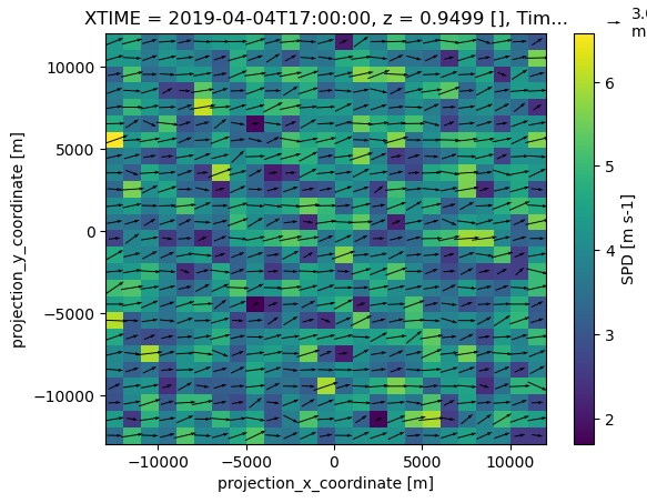
That was a LOT less code!
COGS Cloud Fraction
The Cloud Optically Gridded by Stereo (COGS) data set is very good for cloud fractions <0.5. How does the the COGS cloud fraction compare to this simulation?
Let’s open one of the COGS obs-mod files to see how the hourly data is stored in these files. They contain both the observation and model values on aligned coordinates. Note the “source_type” coordinate’s attribute.
source_type == 0 is the processed observations
source_type == 1 is the processed model output
# We will use the processed, hourly cloud fraction data from the sgplassocogsdiagobsmod datastream.
ds_cogs = xr.open_dataset(f"{path_shcu_root}/{case_date:%Y%m%d}/sim{sim_id:04d}/obs_model/sgplassocogsdiagobsmod{sim_id}C1.m1.{case_date:%Y%m%d}.120000.nc")
ds_cogs
<xarray.Dataset> Size: 1kB
Dimensions:                               (time: 16, bound: 2, source_type: 2)
Coordinates:
  * time                                  (time) datetime64[ns] 128B 2019-04-...
  * source_type                           (source_type) int32 8B 0 1
Dimensions without coordinates: bound
Data variables:
    base_time                             datetime64[ns] 8B ...
    time_offset                           (time) datetime64[ns] 128B ...
    time_bounds                           (time, bound) datetime64[ns] 256B ...
    low_cloud_fraction_cogs               (time, source_type) float32 128B ...
    qc_low_cloud_fraction_cogs            (time, source_type) int32 128B ...
    low_cloud_fraction_cogs_goodfraction  (time, source_type) float32 128B ...
    low_cloud_fraction_cogs_std           (time, source_type) float32 128B ...
    lat                                   float32 4B ...
    lon                                   float32 4B ...
    alt                                   float32 4B ...
Attributes: (12/34)
    command_line:                          Not applicable
    Conventions:                           ARM-1.3
    process_version:                       Not applicable
    dod_version:                           lassocogsdiagobsmod4-m1-1.0
    input_datastreams:                     sgplassodiagmod4C1.m1 : 1.1 : 2019...
    site_id:                               sgp
    ...                                    ...
    config_forecast_time:                  15.0 h
    config_boundary_method:                Periodic
    config_microphysics:                   Thompson (mp_physics=8)
    config_nickname:                       runlas20190404v1addhm
    doi:                                   10.5439/1673163
history: created by user ttoto on machine a...- time: 16
- bound: 2
- source_type: 2
- time(time)datetime64[ns]2019-04-04T12:00:00 ... 2019-04-...
- long_name :
- Time offset from midnight
- standard_name :
- time
- bounds :
- time_bounds
array(['2019-04-04T12:00:00.000000000', '2019-04-04T13:00:00.000000000', '2019-04-04T14:00:00.000000000', '2019-04-04T15:00:00.000000000', '2019-04-04T16:00:00.000000000', '2019-04-04T17:00:00.000000000', '2019-04-04T18:00:00.000000000', '2019-04-04T19:00:00.000000000', '2019-04-04T20:00:00.000000000', '2019-04-04T21:00:00.000000000', '2019-04-04T22:00:00.000000000', '2019-04-04T23:00:00.000000000', '2019-04-05T00:00:00.000000000', '2019-04-05T01:00:00.000000000', '2019-04-05T02:00:00.000000000', '2019-04-05T03:00:00.000000000'], dtype='datetime64[ns]') - source_type(source_type)int320 1
- long_name :
- Type of data source
- units :
- 1
- flag_values :
- [0 1]
- flag_meanings :
- Observation Model
- flag_0_description :
- Observation
- flag_1_description :
- Model
array([0, 1], dtype=int32)
- base_time()datetime64[ns]...
- string :
- 2019-04-04 00:00:00 0:00
- long_name :
- Base time in Epoch
- ancillary_variables :
- time_offset
[1 values with dtype=datetime64[ns]]
- time_offset(time)datetime64[ns]...
- long_name :
- Time offset from base_time
- ancillary_variables :
- base_time
[16 values with dtype=datetime64[ns]]
- time_bounds(time, bound)datetime64[ns]...
- long_name :
- Time cell bounds
- bound_offsets :
- [-1800. 1800.]
[32 values with dtype=datetime64[ns]]
- low_cloud_fraction_cogs(time, source_type)float32...
- long_name :
- Cloud fraction as identified by COGS
- units :
- 1
- valid_min :
- 0.0
- valid_max :
- 1.0
- cell_methods :
- time: mean
- ancillary_variables :
- qc_low_cloud_fraction_cogs low_cloud_fraction_cogs_goodfraction low_cloud_fraction_cogs_std
- resolution :
- 1e-04
[32 values with dtype=float32]
- qc_low_cloud_fraction_cogs(time, source_type)int32...
- long_name :
- Quality check results on variable: Cloud fraction as identified by COGS
- units :
- 1
- description :
- This variable contains bit-packed integer values, where each bit represents a QC test on the data. Non-zero bits indicate the QC condition given in the description for those bits; a value of 0 (no bits set) indicates the data has not failed any QC tests.
- flag_method :
- bit
- bit_1_description :
- Calculated with valid points between 30% and 50%
- bit_1_assessment :
- Indeterminate
- bit_2_description :
- Calculated with valid points less than 30%
- bit_2_assessment :
- Bad
- standard_name :
- quality_flag
[32 values with dtype=int32]
- low_cloud_fraction_cogs_goodfraction(time, source_type)float32...
- long_name :
- Metric goodfraction for Cloud fraction as identified by COGS
- units :
- 1
- resolution :
- 0.001
[32 values with dtype=float32]
- low_cloud_fraction_cogs_std(time, source_type)float32...
- long_name :
- Metric standard deviation for field Cloud fraction as identified by COGS
- units :
- 1
- resolution :
- 1e-04
- cell_methods :
- time: standard_deviation
[32 values with dtype=float32]
- lat()float32...
- long_name :
- North latitude
- units :
- degree_N
- valid_min :
- -90.0
- valid_max :
- 90.0
- standard_name :
- latitude
[1 values with dtype=float32]
- lon()float32...
- long_name :
- East longitude
- units :
- degree_E
- valid_min :
- -180.0
- valid_max :
- 180.0
- standard_name :
- longitude
[1 values with dtype=float32]
- alt()float32...
- long_name :
- Altitude above mean sea level
- units :
- m
- standard_name :
- altitude
[1 values with dtype=float32]
- timePandasIndex
PandasIndex(DatetimeIndex(['2019-04-04 12:00:00', '2019-04-04 13:00:00', '2019-04-04 14:00:00', '2019-04-04 15:00:00', '2019-04-04 16:00:00', '2019-04-04 17:00:00', '2019-04-04 18:00:00', '2019-04-04 19:00:00', '2019-04-04 20:00:00', '2019-04-04 21:00:00', '2019-04-04 22:00:00', '2019-04-04 23:00:00', '2019-04-05 00:00:00', '2019-04-05 01:00:00', '2019-04-05 02:00:00', '2019-04-05 03:00:00'], dtype='datetime64[ns]', name='time', freq=None)) - source_typePandasIndex
PandasIndex(Index([0, 1], dtype='int32', name='source_type'))
- command_line :
- Not applicable
- Conventions :
- ARM-1.3
- process_version :
- Not applicable
- dod_version :
- lassocogsdiagobsmod4-m1-1.0
- input_datastreams :
- sgplassodiagmod4C1.m1 : 1.1 : 20190404.12000; COGS PI Product Data: sgpcldfraccogs01mC1.c1.20190404.000030.nc sgpcldfraccogs01mC1.c1.20190405.000030.nc
- site_id :
- sgp
- platform_id :
- Not applicable
- facility_id :
- C1
- location_description :
- Southern Great Plains (SGP), Lamont, Oklahoma
- contacts :
- lasso@arm.gov, LASSO PI: William Gustafson (William.Gustafson@pnnl.gov), LASSO Co-PI: Andrew Vogelmann (vogelmann@bnl.gov)
- data_level :
- m1
- datastream :
- lassocogsdiagobsmod4
- simulation_id_number :
- 4
- simulation_origin_host :
- cumulus-login2.ccs.ornl.gov
- model_type :
- WRF
- model_version :
- 3.8.1
- model_github_hash :
- b6b6a5cc4229eec1ea9b005746b5ebef2205fb07
- output_domain_size :
- 25.0 km
- output_number_of_levels :
- 226
- output_horizontal_grid_spacing :
- 100 m
- config_large_scale_forcing :
- ECMWF
- config_large_scale_forcing_scale :
- 114 km
- config_large_scale_forcing_specifics :
- sgpecmwfvarX1.c1,sgpecmwftenX1.c1,sgpecmwfsfc1lX1.c1,sgpecmwfsfceX1.c1 (v20191206)
- config_surface_treatment :
- VARANAL
- config_surface_treatment_specifics :
- sgp60varanarapC1.c1 (v20191126)
- config_initial_condition :
- Sounding
- config_initial_condition_specifics :
- sgpsondewnpnC1
- config_aerosol :
- NA
- config_forecast_time :
- 15.0 h
- config_boundary_method :
- Periodic
- config_microphysics :
- Thompson (mp_physics=8)
- config_nickname :
- runlas20190404v1addhm
- doi :
- 10.5439/1673163
- history :
- created by user ttoto on machine agate at 2020-06-11 17:05:43, using vap-lassodiagobsmod-2.0-0.el7 ; modified on 2021-04-28 19:23:05 to contain COGS CF instead of ARSCL CF
Plotting these side-by-side is now easy since everything is aligned and sampled similarly.
fig, ax = plt.subplots(ncols=1)

# These two lines are all you really need for a quick-and-dirty plot...
ds_cogs["low_cloud_fraction_cogs"].isel(source_type=0).plot(ax=ax, marker="o", label="COGS")
ds_cogs["low_cloud_fraction_cogs"].isel(source_type=1).plot(ax=ax, marker="o", label="wrfstat")

# If you plan to share with frieds, do a little clean-up beyond the default labelling from xarray...
ax.legend()
ax.set_title("COGS vs. WRF Cloud Fraction")
ax.set_xlabel("Time (UTC)")
ax.set_ylabel("Cloud Fraction")

plt.show()
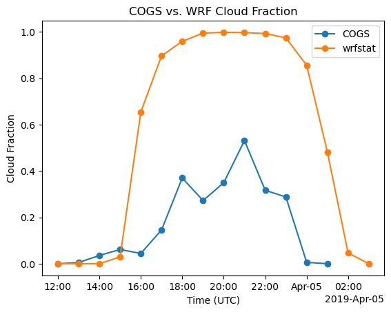
List of LASSO-ShCu data pre-staged for the 2024 ARM Summer School
Selected simulations for 4-Apr-2019 and 5-May-2019 with all four LASSO-ShCu file types:
sgplassodiagconfobsmod,sgplassodiagraw,sgplassocogsdiagobsmod, andsgplassohighfreqobsWe are working to get addtitional 2019 simulations online.
Staged path of Wolf2: /gpfs/wolf2/arm/atm124/world-shared/arm-summer-school-2024/lasso_tutorial/ShCu/untar
Staged path on Jupyter: TBD