Introduction to Xarray

Overview

This notebook will introduce the basics of gridded, labeled data with Xarray. Since Xarray introduces additional abstractions on top of plain arrays of data, our goal is to show why these abstractions are useful and how they frequently lead to simpler, more robust code.

We’ll cover these topics:

Create a DataArray, one of the core object types in Xarray
Understand how to use named coordinates and metadata in a DataArray
Combine individual DataArrays into a Dataset, the other core object type in Xarray
Subset, slice, and interpolate the data using named coordinates
Open netCDF data using XArray
Basic subsetting and aggregation of a Dataset
Brief introduction to plotting with Xarray

Prerequisites

Concepts	Importance	Notes
NumPy Basics	Necessary
Intermediate NumPy	Helpful	Familiarity with indexing and slicing arrays
NumPy Broadcasting	Helpful	Familiar with array arithmetic and broadcasting
Introduction to Pandas	Helpful	Familiarity with labeled data
Datetime	Helpful	Familiarity with time formats and the `timedelta` object
Understanding of NetCDF	Helpful	Familiarity with metadata structure

Time to learn: 30 minutes

Imports

Simmilar to numpy, np; pandas, pd; you may often encounter xarray imported within a shortened namespace as xr.

from datetime import timedelta

import cmweather
import numpy as np
import pandas as pd
import xarray as xr
import glob

from bokeh.models.formatters import DatetimeTickFormatter
import hvplot.xarray
import holoviews as hv
hv.extension("bokeh")

Plotting with Xarray

Another major benefit of using labeled data structures is that they enable automated plotting with sensible axis labels.

Simple visualization with `.plot()`

Much like we saw in Pandas, Xarray includes an interface to Matplotlib that we can access through the .plot() method of every DataArray.

For quick and easy data exploration, we can just call .plot() without any modifiers:

prof.plot();

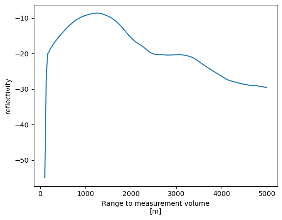
../../_images/d705e44ee523b455f197555391e3726af126c28974e2ad7c6ebe289788573ca1.png

Here Xarray has generated a line plot of the temperature data against the coordinate variable isobaric. Also the metadata are used to auto-generate axis labels and units.

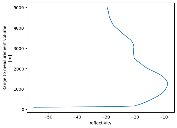
Customizing the plot

As in Pandas, the .plot() method is mostly just a wrapper to Matplotlib, so we can customize our plot in familiar ways.

In this air temperature profile example, we would like to make two changes:

swap the axes so that we have isobaric levels on the y (vertical) axis of the figure
make pressure decrease upward in the figure, so that up is up

A few keyword arguments to our .plot() call will take care of this:

prof.plot(y="range")

[<matplotlib.lines.Line2D at 0x29c367d50>]

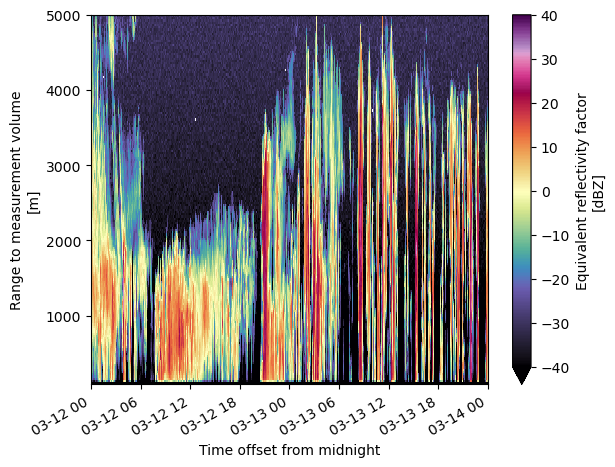
../../_images/307b454bce3f36406ac103c48a27be53b6bebc2bc73fd999f0fa1eedc257a462.png

Plotting 2D data

In the example above, the .plot() method produced a line plot.

What if we call .plot() on a 2D array?

ref.sel(range=slice(0, 5000)).plot(y='range',
                                   cmap='ChaseSpectral',
                                   vmin=-40,
                                   vmax=40)

<matplotlib.collections.QuadMesh at 0x2a6600590>

../../_images/f634b7590ead34242b57a4695b65ab89c8929b6c1786c194b8e680d2bf39cca1.png

We can also make this interactive!

ref.sel(range=slice(0, 5000)).hvplot(x='time',
                                     y='range',
                                     cmap='ChaseSpectral',
                                     clim=(-20, 40),
                                     rasterize=True)

WARNING:param.Image04834: Image dimension time is  not evenly sampled to relative tolerance of 0.001. Please use the QuadMesh element for irregularly sampled data or set a higher tolerance on hv.config.image_rtol or the rtol parameter in the Image constructor.
WARNING:param.Image04834: Image dimension time is  not evenly sampled to relative tolerance of 0.001. Please use the QuadMesh element for irregularly sampled data or set a higher tolerance on hv.config.image_rtol or the rtol parameter in the Image constructor.

ds.reflectivity.sel(range=slice(0, 5000)).plot(y='range', cmap='Spectral_r');

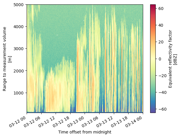
../../_images/436728774d31de7b7fc4649a0f460065016da19b8b4431f1f1b807791a5a80f0.png

ds.reflectivity.sel(range=slice(0, 5000)).hvplot(x='time', y='range', cmap='Spectral_r', rasterize=True, clabel='Reflectivity (dBZ)')

WARNING:param.Image06073: Image dimension time is  not evenly sampled to relative tolerance of 0.001. Please use the QuadMesh element for irregularly sampled data or set a higher tolerance on hv.config.image_rtol or the rtol parameter in the Image constructor.
WARNING:param.Image06073: Image dimension time is  not evenly sampled to relative tolerance of 0.001. Please use the QuadMesh element for irregularly sampled data or set a higher tolerance on hv.config.image_rtol or the rtol parameter in the Image constructor.

Customize our Interactive Plots

Our time axis doesn’t tell us much… we can change that! Also note that we add additional parameters to customize our view of the field.

formatter = DatetimeTickFormatter(hours="%d %b %Y \n %H:%M UTC")
reflectivity_plot = ds.reflectivity.sel(range=slice(0, 5000)).hvplot(x='time', y='range', cmap='Spectral_r', xformatter=formatter, clim=(-20, 40), rasterize=True, clabel='Reflectivity (dBZ)')
reflectivity_plot

WARNING:param.Image06893: Image dimension time is  not evenly sampled to relative tolerance of 0.001. Please use the QuadMesh element for irregularly sampled data or set a higher tolerance on hv.config.image_rtol or the rtol parameter in the Image constructor.
WARNING:param.Image06893: Image dimension time is  not evenly sampled to relative tolerance of 0.001. Please use the QuadMesh element for irregularly sampled data or set a higher tolerance on hv.config.image_rtol or the rtol parameter in the Image constructor.

And the same for velocity…

velocity_plot = ds.mean_doppler_velocity.sel(range=slice(0, 5000)).hvplot(x='time', y='range', cmap='seismic', xformatter=formatter, clim=(-5, 5), rasterize=True, clabel='Mean Doppler Velocity (m/s)')
velocity_plot

WARNING:param.Image07300: Image dimension time is  not evenly sampled to relative tolerance of 0.001. Please use the QuadMesh element for irregularly sampled data or set a higher tolerance on hv.config.image_rtol or the rtol parameter in the Image constructor.
WARNING:param.Image07300: Image dimension time is  not evenly sampled to relative tolerance of 0.001. Please use the QuadMesh element for irregularly sampled data or set a higher tolerance on hv.config.image_rtol or the rtol parameter in the Image constructor.

Combine our Plots

Now that we have our interactive plots, we can combine them using +

reflectivity_plot + velocity_plot

Or stacked on top of each other…

(reflectivity_plot + velocity_plot).cols(1)

Summary

Xarray brings the joy of Pandas-style labeled data operations to N-dimensional data. As such, it has become a central workhorse in the geoscience community for the analysis of gridded datasets. Xarray allows us to open self-describing NetCDF files and make full use of the coordinate axes, labels, units, and other metadata. By making use of labeled coordinates, our code is often easier to write, easier to read, and more robust.

We also covered some interactive plots using xarray and hvPlot!

What’s next?

Additional notebooks to appear in this section will go into more detail about

arithemtic and broadcasting with Xarray data structures
using “group by” operations
remote data access with OpenDAP
more advanced visualization including map integration with Cartopy

Resources and references

This notebook was adapated from material in Unidata’s Python Training.

The best resource for Xarray is the Xarray documentation. See in particular

Another excellent resource is this Xarray Tutorial collection.

Introduction to Xarray

Contents

Introduction to Xarray

Overview

Prerequisites

Imports

Introducing the DataArray and Dataset

Creation of a DataArray object

Generate a random numpy array

Wrap the array: first attempt

Assign dimension names

Create a DataArray with named Coordinates

Make time and space coordinates

Initialize the DataArray with complete coordinate info

Set useful attributes

Attributes are not preserved by default!

The Dataset: a container for DataArrays with shared coordinates

Create a pressure DataArray using the same coordinates

Create a Dataset object

Access Data variables and Coordinates in a Dataset

Subsetting and selection by coordinate values

NumPy-like selection

Selecting with .sel()

Approximate selection and interpolation

Nearest-neighbor sampling

Interpolation

Slicing along coordinates

One more selection method: .loc

Opening netCDF data

Access netCDF data with xr.open_dataset

Read in Multiple Files Using open_mfdataset

Subsetting the Dataset

Aggregation operations

Plotting with Xarray

Simple visualization with .plot()

Customizing the plot

Plotting 2D data

Customize our Interactive Plots

Combine our Plots

Summary

What’s next?

Resources and references

Introducing the `DataArray` and `Dataset`

Creation of a `DataArray` object

Create a `DataArray` with named Coordinates

Initialize the `DataArray` with complete coordinate info

The `Dataset`: a container for `DataArray`s with shared coordinates

Create a pressure `DataArray` using the same coordinates

Create a `Dataset` object

Access Data variables and Coordinates in a `Dataset`

Selecting with `.sel()`

One more selection method: `.loc`

Access netCDF data with `xr.open_dataset`

Read in Multiple Files Using `open_mfdataset`

Subsetting the `Dataset`

Simple visualization with `.plot()`