![]()
Solutions: Snowfall Retrievals from SAIL X-Band Radar
%env PYTHONWARNINGS=ignore
env: PYTHONWARNINGS=ignore
import warnings
warnings.filterwarnings("ignore", category=DeprecationWarning)
warnings.filterwarnings("ignore", category=UserWarning)

import glob
import os
import datetime

import numpy as np
import matplotlib.pyplot as plt
import pyart
import act
import xarray as xr
from matplotlib.dates import DateFormatter
from pathlib import Path

from metpy.plots import USCOUNTIES
from dask.distributed import Client, LocalCluster

import cartopy.crs as ccrs
import cartopy.feature as cfeature

import xwrf
## You are using the Python ARM Radar Toolkit (Py-ART), an open source
## library for working with weather radar data. Py-ART is partly
## supported by the U.S. Department of Energy as part of the Atmospheric
## Radiation Measurement (ARM) Climate Research Facility, an Office of
## Science user facility.
##
## If you use this software to prepare a publication, please cite:
##
##     JJ Helmus and SM Collis, JORS 2016, doi: 10.5334/jors.119
ERROR 1: PROJ: proj_create_from_database: Open of /opt/conda/share/proj failed
Setup Helper Functions
We setup helper functions to calculate the snowfall retrieval, using following notation:
\(Z = A*S ^ {B}\)
Where:
Z = Reflectivity in dBZ
A = Coefficient applied to Z-S Relationship (not in the exponent)
S = Liquid snowfall rate
B = Coefficient applied to Z-S Relationship (in the exponent)
We also need to apply a snow water equivalent ratio (swe) to convert from liquid to snow (ex. 8 inches of snow –> 1 inch of rain would be 8.0).
This equation now becomes:
\(Z = swe*A*S ^ {B}\)
Solving for S, we get:
\(S = swe * (\frac{z}{a})^{1/B}\)
Where z is reflectivity in units of dB (\(z =10^{Z/10}\))
List the Available Files
We will use files on the Oak Ridge Laboratory Computing Facility (ORLCF), within the shared SAIL directory /gpfs/wolf/atm124/proj-shared/sail.
file_list = sorted(glob.glob("/data/project/ARM_Summer_School_2024_Data/sail/radar/*"))
file_list[0:10]
['/data/project/ARM_Summer_School_2024_Data/sail/radar/gucxprecipradarcmacS2.c1.20220310.000206.nc',
 '/data/project/ARM_Summer_School_2024_Data/sail/radar/gucxprecipradarcmacS2.c1.20220310.000726.nc',
 '/data/project/ARM_Summer_School_2024_Data/sail/radar/gucxprecipradarcmacS2.c1.20220310.001246.nc',
 '/data/project/ARM_Summer_School_2024_Data/sail/radar/gucxprecipradarcmacS2.c1.20220310.001806.nc',
 '/data/project/ARM_Summer_School_2024_Data/sail/radar/gucxprecipradarcmacS2.c1.20220310.002326.nc',
 '/data/project/ARM_Summer_School_2024_Data/sail/radar/gucxprecipradarcmacS2.c1.20220310.002846.nc',
 '/data/project/ARM_Summer_School_2024_Data/sail/radar/gucxprecipradarcmacS2.c1.20220310.003406.nc',
 '/data/project/ARM_Summer_School_2024_Data/sail/radar/gucxprecipradarcmacS2.c1.20220310.003926.nc',
 '/data/project/ARM_Summer_School_2024_Data/sail/radar/gucxprecipradarcmacS2.c1.20220310.004446.nc',
 '/data/project/ARM_Summer_School_2024_Data/sail/radar/gucxprecipradarcmacS2.c1.20220310.005006.nc']
Question 1 - Easy
Using material presented this week, apply one of the above relationships to SAIL X-Band radar file and display
Read Data + Apply Snowfall Retrieval
def snow_rate(radar, swe_ratio, A, B, key="snow_z"):
    """
    Snow rate applied to a pyart.Radar object

    Takes a given Snow Water Equivilent ratio (swe_ratio), A and B value
    for the Z-S relationship and creates a radar field similar to DBZ
    showing the radar estimated snowfall rate in mm/hr. Then the given
    SWE_ratio, A and B are stored in the radar metadata for later
    reference.

    """
    # Setting up for Z-S relationship:
    snow_z = radar.fields['corrected_reflectivity']['data'].copy()
    # Convert it from dB to linear units
    z_lin = 10.0**(radar.fields['corrected_reflectivity']['data']/10.)
    # Apply the Z-S relation.
    snow_z = swe_ratio * (z_lin/A)**(1./B)
    # Add the field back to the radar. Use reflectivity as a template
    radar.add_field_like('corrected_reflectivity', key,  snow_z,
                         replace_existing=True)
    # Update units and metadata
    radar.fields[key]['units'] = 'mm/h'
    radar.fields[key]['standard_name'] = 'snowfall_rate'
    radar.fields[key]['long_name'] = 'user_defined_snowfall_rate_from_z'
    radar.fields[key]['valid_min'] = 0
    radar.fields[key]['valid_max'] = 500
    radar.fields[key]['swe_ratio'] = swe_ratio
    radar.fields[key]['A'] = A
    radar.fields[key]['B'] = B
    return radar
radar = pyart.io.read(file_list[0])
radar = snow_rate(radar, 8.5, 67, 1.28, key="snow_z_new")
/opt/conda/lib/python3.11/site-packages/numpy/ma/core.py:6980: RuntimeWarning: overflow encountered in power
  result = np.where(m, fa, umath.power(fa, fb)).view(basetype)
# Check to see if the snowfall retrieval was applied
list(radar.fields.keys())
['DBZ',
 'VEL',
 'WIDTH',
 'ZDR',
 'PHIDP',
 'RHOHV',
 'NCP',
 'DBZhv',
 'cbb_flag',
 'sounding_temperature',
 'height',
 'signal_to_noise_ratio',
 'velocity_texture',
 'gate_id',
 'simulated_velocity',
 'corrected_velocity',
 'unfolded_differential_phase',
 'corrected_differential_phase',
 'filtered_corrected_differential_phase',
 'corrected_specific_diff_phase',
 'filtered_corrected_specific_diff_phase',
 'corrected_differential_reflectivity',
 'corrected_reflectivity',
 'height_over_iso0',
 'specific_attenuation',
 'path_integrated_attenuation',
 'specific_differential_attenuation',
 'path_integrated_differential_attenuation',
 'rain_rate_A',
 'snow_rate_ws2012',
 'snow_rate_ws88diw',
 'snow_rate_m2009_1',
 'snow_rate_m2009_2',
 'snow_z_new']
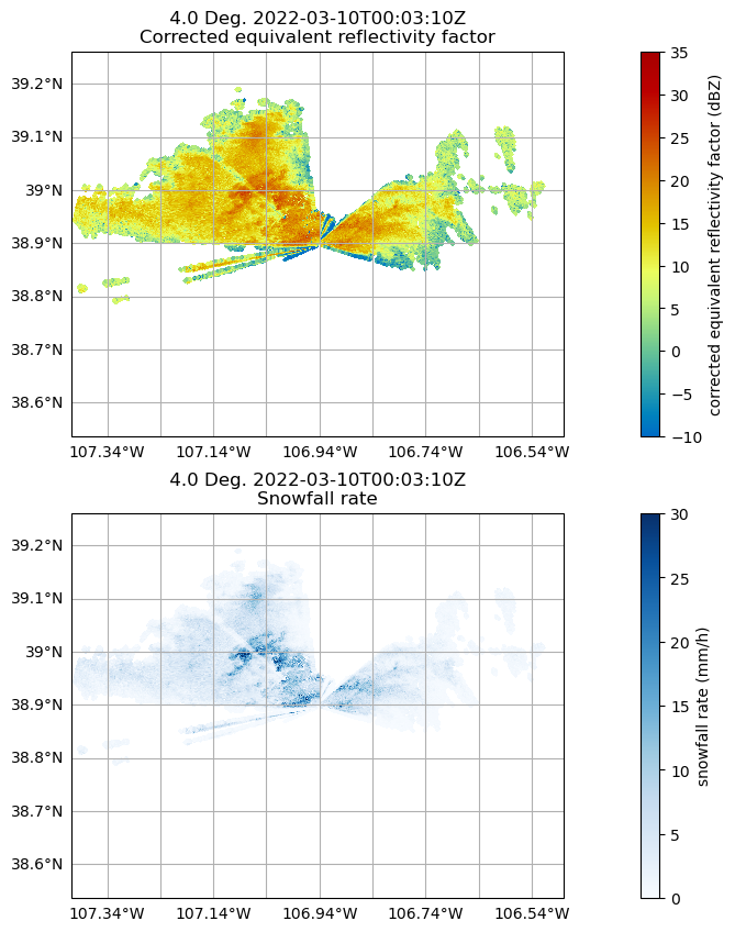
Display Snowfall Retrieval
# Create the Py-ART display object
display = pyart.graph.RadarMapDisplay(radar)
# Define the matplotlib figure
fig = plt.figure(figsize=(18,10))

# Extract the latitude and longitude of the radar and use it for the center of the map
lat_center = round(radar.latitude['data'][0], 2)
lon_center = round(radar.longitude['data'][0], 2)

# Set the projection - in this case, we use a general PlateCarree projection
projection = ccrs.PlateCarree()

# Determine the ticks
lat_ticks = np.arange(lat_center-0.5, lat_center+1, .1)
lon_ticks = np.arange(lon_center-0.5, lon_center+1, .1)

# Define a subplot for the reflectivity field
ax1 = plt.subplot(211, projection=projection)
display.plot_ppi_map("corrected_reflectivity",
                     2,
                     resolution='10m',
                     ax=ax1,
                     lat_lines=lat_ticks,
                     lon_lines=lon_ticks,
                     vmin=-10,
                     vmax=35)

# Define a subplot for the snowfall retrieval
ax2 = plt.subplot(212, projection=projection)
display.plot_ppi_map("snow_z_new",
                     2,
                     resolution='10m',
                     ax=ax2,
                     lat_lines=lat_ticks,
                     lon_lines=lon_ticks,
                     vmin=0,
                     vmax=30,
                     cmap='Blues')
Question 2 - Intermediate
Using the above methodology, calculate the snowfall accumulation for an hour (or day)
Gridded Observations Using Nearest Neighbor Interpolation
def compute_number_of_points(extent, resolution):
    """
    Create a helper function to determine number of points
    """
    return int((extent[1] - extent[0])/resolution)

# Grid extents in meters
z_grid_limits = (500.,5_000.)
y_grid_limits = (-20_000.,20_000.)
x_grid_limits = (-20_000.,20_000.)

# Grid resolution in meters
grid_resolution = 250

# Determine number of points with our desired input
x_grid_points = compute_number_of_points(x_grid_limits, grid_resolution)
y_grid_points = compute_number_of_points(y_grid_limits, grid_resolution)
z_grid_points = compute_number_of_points(z_grid_limits, grid_resolution)

print(z_grid_points,
      y_grid_points,
      x_grid_points)
18 160 160
# Call Py-ART gridding module, with our grid specifications
grid = pyart.map.grid_from_radars(radar,
                                  grid_shape=(z_grid_points,
                                              y_grid_points,
                                              x_grid_points),
                                  grid_limits=(z_grid_limits,
                                               y_grid_limits,
                                               x_grid_limits),
                                  method='nearest'
                                 )
ds = grid.to_xarray()
ds
<xarray.Dataset> Size: 122MB
Dimensions:                                   (time: 1, z: 18, y: 160, x: 160)
Coordinates:
  * time                                      (time) object 8B 2022-03-10 00:...
  * z                                         (z) float64 144B 500.0 ... 5e+03
    lat                                       (y, x) float64 205kB 38.72 ... ...
    lon                                       (y, x) float64 205kB -107.2 ......
  * y                                         (y) float64 1kB -2e+04 ... 2e+04
  * x                                         (x) float64 1kB -2e+04 ... 2e+04
Data variables: (12/35)
    NCP                                       (time, z, y, x) float64 4MB 0.1...
    snow_rate_m2009_1                         (time, z, y, x) float64 4MB nan...
    specific_differential_attenuation         (time, z, y, x) float64 4MB nan...
    filtered_corrected_specific_diff_phase    (time, z, y, x) float64 4MB 0.0...
    path_integrated_differential_attenuation  (time, z, y, x) float64 4MB nan...
    filtered_corrected_differential_phase     (time, z, y, x) float64 4MB 0.0...
    ...                                        ...
    corrected_differential_reflectivity       (time, z, y, x) float64 4MB nan...
    simulated_velocity                        (time, z, y, x) float64 4MB -2....
    rain_rate_A                               (time, z, y, x) float64 4MB nan...
    sounding_temperature                      (time, z, y, x) float32 2MB -13...
    signal_to_noise_ratio                     (time, z, y, x) float64 4MB -1....
ROI (time, z, y, x) float32 2MB 493...ds.snow_z_new.isel(z=0).plot(x='lon',
y='lat',
vmin=0,
vmax=50,
cmap='pyart_HomeyerRainbow')
<matplotlib.collections.QuadMesh at 0x7f0e9ea34510>
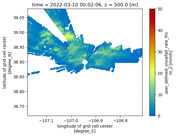
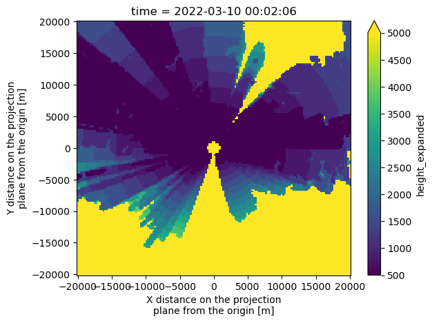
Determine the Lowest Height in Each Column
We plotted the lowest level (500 m) in the plot above. It would be more helpful to have data from the lowest data point (lowest z) in each column (across time, latitude, and longitude)
We start first by creating a new field in our dataset, height_expanded, which is a four-dimensional (time, z, x, y) vertical coordinate, with nan values where we have missing snow rate values.
ds["height_expanded"] = (ds.z * (ds.snow_z_new/ds.snow_z_new)).fillna(10_000)
Next, we find the index of the lowest value in this column, using the .argmin method, looking over the column (z)
min_index = ds.height_expanded.argmin(dim='z',
                                      skipna=True)
Here is a plot of the lowest value height in the column for our domain:
**Notice how some values are the top of the column - 5000 m, whereas some of the values are close lowest vertical level, 500 m
ds.height_expanded.isel(z=min_index).plot(vmin=500,
                                          vmax=5000);
Apply this to our snow fields
We first check for snow fields in our dataset, by using the following list comprehension line:
snow_fields = [var for var in list(ds.variables) if "snow" in var]
snow_fields
['snow_rate_m2009_1',
 'snow_rate_m2009_2',
 'snow_rate_ws88diw',
 'snow_z_new',
 'snow_rate_ws2012']
subset_ds = ds[snow_fields].isel(z=min_index)
Visualize our closest-to-ground snow value
Now that we have the lowest vertical level in each column, let’s plot our revised maps, which only have dimensions:
time
latitude
longitude
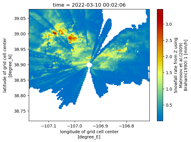
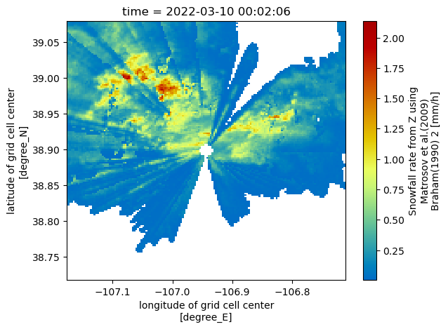
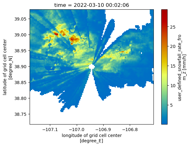
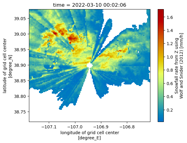
for snow_field in snow_fields:
    subset_ds[snow_field].plot(x='lon',
                               y='lat',
                               cmap='pyart_HomeyerRainbow')
    plt.show()
    plt.close()

Calculate Daily Accumulation of Snowfall
def grid_radar(file,
               x_grid_limits=(-20_000.,20_000.),
               y_grid_limits=(-20_000.,20_000.),
               z_grid_limits = (500.,5_000.),
               grid_resolution = 250,

               ):
    """
    Grid the radar using some provided parameters
    """
    try:
        radar = pyart.io.read(file)
    except:
        radar = None

    if radar:
        x_grid_points = compute_number_of_points(x_grid_limits, grid_resolution)
        y_grid_points = compute_number_of_points(y_grid_limits, grid_resolution)
        z_grid_points = compute_number_of_points(z_grid_limits, grid_resolution)

        grid = pyart.map.grid_from_radars(radar,
                                          grid_shape=(z_grid_points,
                                                      y_grid_points,
                                                      x_grid_points),
                                          grid_limits=(z_grid_limits,
                                                       y_grid_limits,
                                                       x_grid_limits),
                                          method='nearest'
                                         )
        grid_out = grid.to_xarray()
        del radar
    else:
        grid_out = None

    return grid_out

def subset_lowest_vertical_level(ds, additional_fields=["corrected_reflectivity"]):
    """
    Filter the dataset based on the lowest vertical level
    """
    snow_fields = [var for var in list(ds.variables) if "snow" in var] + additional_fields

    # Create a new 4-d height field
    ds["height_expanded"] = (ds.z * (ds[snow_fields[0]]/ds[snow_fields[0]])).fillna(5_000)

    # Find the minimum height index
    min_index = ds.height_expanded.argmin(dim='z',
                                          skipna=True)

    # Subset our snow fields based on this new index
    subset_ds = ds[snow_fields].isel(z=min_index)

    return subset_ds
def process_squire(file):
    """ Script to process SQUIRE """
    ds = grid_radar(file)
    if ds:
        out_ds = subset_lowest_vertical_level(ds)

        # Create an output path
        ##out_path = f"./{Path(file).stem}.gridded.nc"
        ##out_ds.to_netcdf(out_path)

        # free up memory
        del ds
    else:
        out_ds = None

    return out_ds
Spin up Dask Cluster and Process SQUIRE
%%time
## Start up a Dask Cluster
cluster = LocalCluster()
with Client(cluster) as client:
    future = client.map(process_squire, file_list)
    my_data = client.gather(future)
ERROR 1: PROJ: proj_create_from_database: Open of /opt/conda/share/proj failed
ERROR 1: PROJ: proj_create_from_database: Open of /opt/conda/share/proj failed
ERROR 1: PROJ: proj_create_from_database: Open of /opt/conda/share/proj failed
ERROR 1: PROJ: proj_create_from_database: Open of /opt/conda/share/proj failed
2024-05-22 18:33:11,321 - distributed.nanny - WARNING - Restarting worker
2024-05-22 18:33:11,377 - distributed.nanny - WARNING - Restarting worker
2024-05-22 18:33:11,383 - distributed.nanny - WARNING - Restarting worker
ERROR 1: PROJ: proj_create_from_database: Open of /opt/conda/share/proj failed
ERROR 1: PROJ: proj_create_from_database: Open of /opt/conda/share/proj failed
ERROR 1: PROJ: proj_create_from_database: Open of /opt/conda/share/proj failed
2024-05-22 18:33:13,939 - distributed.nanny - WARNING - Restarting worker
ERROR 1: PROJ: proj_create_from_database: Open of /opt/conda/share/proj failed
HDF5-DIAG: Error detected in HDF5 (1.14.3) thread 1:
  #000: H5D.c line 611 in H5Dget_space(): unable to synchronously get dataspace
    major: Dataset
    minor: Can't get value
  #001: H5D.c line 571 in H5D__get_space_api_common(): invalid dataset identifier
    major: Invalid arguments to routine
    minor: Inappropriate type
CPU times: user 9.7 s, sys: 4.61 s, total: 14.3 s
Wall time: 9min 37s
# Concatenate all extracted columns across time dimension to form daily timeseries
ds = xr.concat([data for data in my_data if data], dim='time')
Calculate Daily Accumulation
new_ds = ds.resample(time='h').sum()
new_ds
<xarray.Dataset> Size: 25MB
Dimensions:                 (time: 24, y: 160, x: 160)
Coordinates:
    lat                     (y, x) float64 205kB 38.72 38.72 ... 39.08 39.08
    lon                     (y, x) float64 205kB -107.2 -107.2 ... -106.7 -106.7
  * y                       (y) float64 1kB -2e+04 -1.975e+04 ... 2e+04
  * x                       (x) float64 1kB -2e+04 -1.975e+04 ... 2e+04
  * time                    (time) object 192B 2022-03-10 00:00:00 ... 2022-0...
Data variables:
    snow_rate_ws2012        (time, y, x) float64 5MB 0.0 0.0 0.0 ... 0.0 0.0 0.0
    snow_rate_m2009_1       (time, y, x) float64 5MB 0.0 0.0 0.0 ... 0.0 0.0 0.0
    snow_rate_m2009_2       (time, y, x) float64 5MB 0.0 0.0 0.0 ... 0.0 0.0 0.0
    snow_rate_ws88diw       (time, y, x) float64 5MB 0.0 0.0 0.0 ... 0.0 0.0 0.0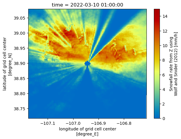
corrected_reflectivity (time, y, x) float64 5MB 0.0 0.0 0.0 ... 0.0 0.0 0.0new_ds['snow_rate_ws2012'].isel(time=1).plot(x='lon', y='lat', cmap='pyart_HomeyerRainbow', vmin=0, vmax=15)
<matplotlib.collections.QuadMesh at 0x7f0e9e02e650>
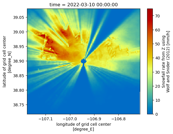
new_ds['snow_rate_ws2012'].resample(time='D').sum().plot(x='lon', y='lat', cmap='pyart_HomeyerRainbow')
<matplotlib.collections.QuadMesh at 0x7f0e9de79f10>
Question 3 - Hard
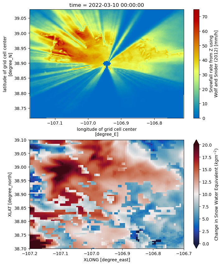
Compare this hourly (or daily) accumulation to WRF output for the same day
Compare against WRF Run
files = sorted(glob.glob("/data/project/ARM_Summer_School_2024_Data/sail/wrf/*"))
first_ds = xr.open_dataset(files[0]).xwrf.postprocess().squeeze()
last_ds = xr.open_dataset(files[-1]).xwrf.postprocess().squeeze()
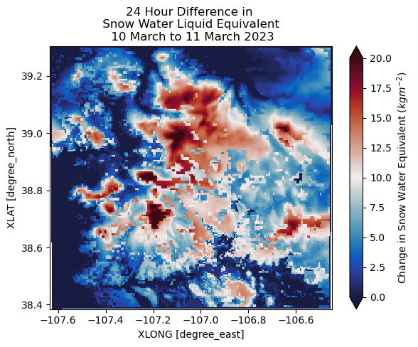
difference = last_ds["SNOW"] - first_ds["SNOW"]
difference.plot(x='XLONG',
                y='XLAT',
                cbar_kwargs={'label': "Change in Snow Water Equivalent ($kgm^{-2}$)"},
                vmin=0,
                vmax=20,
                cmap="pyart_balance")
plt.title("24 Hour Difference in \n Snow Water Liquid Equivalent \n 10 March to 11 March 2023")
Text(0.5, 1.0, '24 Hour Difference in \n Snow Water Liquid Equivalent \n 10 March to 11 March 2023')
fig, axarr = plt.subplots(2, 1, figsize=[8, 10])

new_ds['snow_rate_ws2012'].resample(time='D').sum().plot(x='lon',
                                                         y='lat',
                                                         cmap='pyart_HomeyerRainbow',
                                                         ax=axarr[0])
difference.plot(x='XLONG',
                y='XLAT',
                cbar_kwargs={'label': "Change in Snow Water Equivalent ($kgm^{-2}$)"},
                vmin=0,
                vmax=20,
                cmap="pyart_balance",
                ax=axarr[1])
#axarr[0].set_xlim([-107.7, -106.5])
axarr[1].set_xlim([-107.2, -106.7])
axarr[1].set_ylim([38.7, 39.1])
(38.7, 39.1)