
Py-ART Basics#
Overview#
Within this notebook, we will cover:
General overview of Py-ART and its functionality
Reading data using Py-ART
An overview of the
pyart.RadarobjectCreate a Plot of our Radar Data
Prerequisites#
Concepts |
Importance |
Notes |
|---|---|---|
Helpful |
Basic features |
|
Helpful |
Basic plotting |
|
Helpful |
Basic arrays |
Time to learn: 30 minutes
Imports#
import os
import warnings

import cartopy.crs as ccrs
import matplotlib.pyplot as plt
import numpy as np


import pyart

warnings.filterwarnings('ignore')
## You are using the Python ARM Radar Toolkit (Py-ART), an open source
## library for working with weather radar data. Py-ART is partly
## supported by the U.S. Department of Energy as part of the Atmospheric
## Radiation Measurement (ARM) Climate Research Facility, an Office of
## Science user facility.
##
## If you use this software to prepare a publication, please cite:
##
##     JJ Helmus and SM Collis, JORS 2016, doi: 10.5334/jors.119
/Users/mgrover/miniforge3/envs/pyart-docs/lib/python3.10/site-packages/tqdm/auto.py:22: TqdmWarning: IProgress not found. Please update jupyter and ipywidgets. See https://ipywidgets.readthedocs.io/en/stable/user_install.html
  from .autonotebook import tqdm as notebook_tqdm
An Overview of Py-ART#
History of the Py-ART#
Development began to address the needs of ARM with the acquisition of a number of new scanning cloud and precipitation radar as part of the American Recovery Act.
The project has since expanded to work with a variety of weather radars and a wider user base including radar researchers and climate modelers.
The software has been released on GitHub as open source software under a BSD license. Runs on Linux, OS X. It also runs on Windows with more limited functionality.
What can PyART Do?#
Py-ART can be used for a variety of tasks from basic plotting to more complex processing pipelines. Specific uses for Py-ART include:
Reading radar data in a variety of file formats.
Creating plots and visualization of radar data.
Correcting radar moments while in antenna coordinates, such as:
Doppler unfolding/de-aliasing.
Attenuation correction.
Phase processing using a Linear Programming method.
Mapping data from one or multiple radars onto a Cartesian grid.
Performing retrievals.
Writing radial and Cartesian data to NetCDF files.
Reading in Data Using Py-ART#
The Sample Data - SAIL!#

Our Radar 📡#
Reading data in using pyart.io.read#
When reading in a radar file, we use the pyart.io.read module.
pyart.io.read can read a variety of different radar formats, such as Cf/Radial, LASSEN, and more.
The documentation on what formats can be read by Py-ART can be found here:
For most file formats listed on the page, using pyart.io.read should suffice since Py-ART has the ability to automatically detect the file format.
Let’s check out what arguments arguments pyart.io.read() takes in!
pyart.io.read?
Signature: pyart.io.read(filename, use_rsl=False, **kwargs)
Docstring:
Read a radar file and return a radar object.

Additional parameters are passed to the underlying read_* function.

Parameters
----------
filename : str
    Name of radar file to read.
use_rsl : bool
    True will use the TRMM RSL library to read files which are supported
    both natively and by RSL. False will choose the native read function.
    RSL will always be used to read a file if it is not supported
    natively.

Other Parameters
-------------------
field_names : dict, optional
    Dictionary mapping file data type names to radar field names. If a
    data type found in the file does not appear in this dictionary or has
    a value of None it will not be placed in the radar.fields dictionary.
    A value of None, the default, will use the mapping defined in the
    metadata configuration file.
additional_metadata : dict of dicts, optional
    Dictionary of dictionaries to retrieve metadata from during this read.
    This metadata is not used during any successive file reads unless
    explicitly included. A value of None, the default, will not
    introduct any addition metadata and the file specific or default
    metadata as specified by the metadata configuration file will be used.
file_field_names : bool, optional
    True to use the file data type names for the field names. If this
    case the field_names parameter is ignored. The field dictionary will
    likely only have a 'data' key, unless the fields are defined in
    `additional_metadata`.
exclude_fields : list or None, optional
    List of fields to exclude from the radar object. This is applied
    after the `file_field_names` and `field_names` parameters.
delay_field_loading : bool
    True to delay loading of field data from the file until the 'data'
    key in a particular field dictionary is accessed. In this case
    the field attribute of the returned Radar object will contain
    LazyLoadDict objects not dict objects. Not all file types support this
    parameter.

Returns
-------
radar : Radar
    Radar object. A TypeError is raised if the format cannot be
    determined.
File:      ~/git_repos/pyart/pyart/io/auto_read.py
Type:      function
Let’s use a sample data file from pyart - which is cfradial format.
When we read this in, we get a pyart.Radar object!
file = '../data/sample_sail_ppi.nc'
radar = pyart.io.read(file)
radar
<pyart.core.radar.Radar at 0x283fa3160>
Investigate the pyart.Radar object#
Within this pyart.Radar object object are the actual data fields.
This is where data such as reflectivity and velocity are stored.
To see what fields are present we can add the fields and keys additions to the variable where the radar object is stored.
radar.fields.keys()
dict_keys(['corrected_velocity', 'corrected_reflectivity', 'corrected_differential_reflectivity', 'corrected_specific_diff_phase', 'corrected_differential_phase'])
Extract a sample data field#
The fields are stored in a dictionary, each containing coordinates, units and more. All can be accessed by just adding the fields addition to the radar object variable.
For an individual field, we add a string in brackets after the fields addition to see the contents of that field.
Let’s take a look at 'corrected_reflectivity', which is a common field to investigate.
print(radar.fields['corrected_reflectivity'])
{'_FillValue': 1e+20, 'long_name': 'Corrected reflectivity', 'units': 'dBZ', 'standard_name': 'corrected_equivalent_reflectivity_factor', 'coordinates': 'elevation azimuth range', 'data': masked_array(
  data=[[--, --, --, ..., --, --, --],
        [--, --, --, ..., --, --, --],
        [--, --, --, ..., --, --, --],
        ...,
        [12.25, 9.84000015258789, 14.210000038146973, ..., --, --, --],
        [11.5, 9.729999542236328, 11.75999927520752, ..., --, --, --],
        [11.069999694824219, 10.329999923706055, 10.050000190734863, ...,
         --, --, --]],
  mask=[[ True,  True,  True, ...,  True,  True,  True],
        [ True,  True,  True, ...,  True,  True,  True],
        [ True,  True,  True, ...,  True,  True,  True],
        ...,
        [False, False, False, ...,  True,  True,  True],
        [False, False, False, ...,  True,  True,  True],
        [False, False, False, ...,  True,  True,  True]],
  fill_value=1e+20)}
We can go even further in the dictionary and access the actual reflectivity data.
We use add 'data' at the end, which will extract the data array (which is a masked numpy array) from the dictionary.
reflectivity = radar.fields['corrected_reflectivity']['data']
print(type(reflectivity), reflectivity)
<class 'numpy.ma.core.MaskedArray'> [[-- -- -- ... -- -- --]
 [-- -- -- ... -- -- --]
 [-- -- -- ... -- -- --]
 ...
 [12.25 9.84000015258789 14.210000038146973 ... -- -- --]
 [11.5 9.729999542236328 11.75999927520752 ... -- -- --]
 [11.069999694824219 10.329999923706055 10.050000190734863 ... -- -- --]]
Lets’ check the size of this array…
reflectivity.shape
(9013, 668)
This reflectivity data array, numpy array, is a two-dimensional array with dimensions:
Gates (number of samples away from the radar)
Rays (direction around the radar)
print(radar.nrays, radar.ngates)
9013 668
If we wanted to look the 300th ray, at the second gate, we would use something like the following:
print(reflectivity[300, 2])
9.369999885559082
Plotting our Radar Data#
An Overview of Py-ART Plotting Utilities#
Now that we have loaded the data and inspected it, the next logical thing to do is to visualize the data! Py-ART’s visualization functionality is done through the objects in the pyart.graph module.
In Py-ART there are 4 primary visualization classes in pyart.graph:
Plotting grid data
Use the RadarMapDisplay with our data#
For the this example, we will be using RadarMapDisplay, using Cartopy to deal with geographic coordinates.
We start by creating a figure first.
fig = plt.figure(figsize=[10, 10])
<Figure size 1000x1000 with 0 Axes>
Once we have a figure, let’s add our RadarMapDisplay
fig = plt.figure(figsize=[10, 10])
display = pyart.graph.RadarMapDisplay(radar)
<Figure size 1000x1000 with 0 Axes>
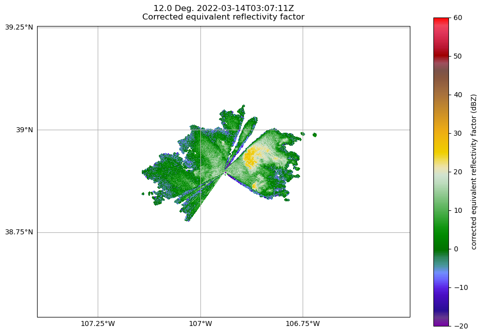
Adding our map display without specifying a field to plot won’t do anything we need to specifically add a field to field using .plot_ppi_map(), which creates a Plan Position Indicator (PPI) plot.
display.plot_ppi_map('corrected_reflectivity')
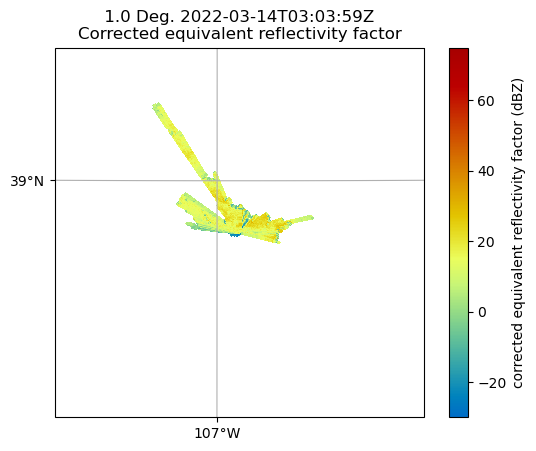
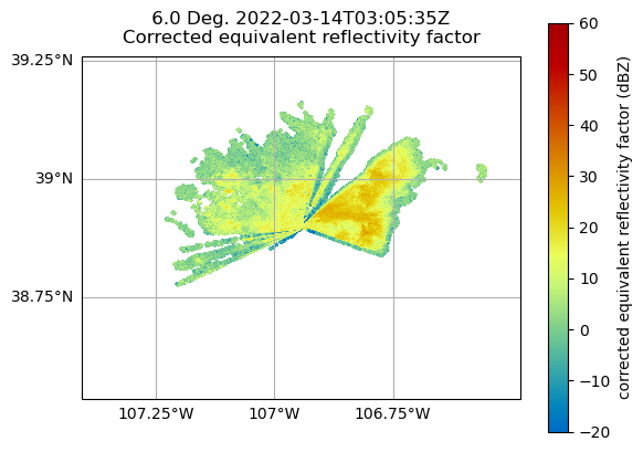
By default, it will plot the elevation scan, the the default colormap from Matplotlib… let’s customize!
We add the following arguements:
sweep=3- The fourth elevation scan (since we are using Python indexing)vmin=-20- Minimum value for our plotted field/colorbarvmax=60- Maximum value for our plotted field/colorbarprojection=ccrs.PlateCarree()- Cartopy latitude/longitude coordinate systemcmap='pyart_HomeyerRainbow'- Colormap to use, selecting one provided by PyART oflat_lines- Which lines to plot for latitudelon_lines- Which liens to plot for longitude
###### fig = plt.figure(figsize=[12, 8])
display = pyart.graph.RadarMapDisplay(radar)
display.plot_ppi_map('corrected_reflectivity',
                     sweep=3,
                     vmin=-20,
                     vmax=60,
                     lat_lines = np.arange(38, 39.5, .25),
                     lon_lines = np.arange(-107.5, -106.5, .25),
                     projection=ccrs.PlateCarree(),
                     cmap='pyart_HomeyerRainbow')
plt.savefig("sample-ppi-map.png", dpi=300)
You can change many parameters in the graph by changing the arguments to plot_ppi_map. As you can recall from earlier. simply view these arguments in a Jupyter notebook by typing:
display.plot_ppi_map?
Signature:
display.plot_ppi_map(
    field,
    sweep=0,
    mask_tuple=None,
    vmin=None,
    vmax=None,
    cmap=None,
    norm=None,
    mask_outside=False,
    title=None,
    title_flag=True,
    colorbar_flag=True,
    colorbar_label=None,
    ax=None,
    fig=None,
    lat_lines=None,
    lon_lines=None,
    projection=None,
    min_lon=None,
    max_lon=None,
    min_lat=None,
    max_lat=None,
    width=None,
    height=None,
    lon_0=None,
    lat_0=None,
    resolution='110m',
    shapefile=None,
    shapefile_kwargs=None,
    edges=True,
    gatefilter=None,
    filter_transitions=True,
    embellish=True,
    raster=False,
    ticks=None,
    ticklabs=None,
    alpha=None,
    edgecolors='face',
    **kwargs,
)
Docstring:
Plot a PPI volume sweep onto a geographic map.

Parameters
----------
field : str
    Field to plot.
sweep : int, optional
    Sweep number to plot.

Other Parameters
----------------
mask_tuple : (str, float)
    Tuple containing the field name and value below which to mask
    field prior to plotting, for example to mask all data where
    NCP < 0.5 set mask_tuple to ['NCP', 0.5]. None performs no masking.
vmin : float
    Luminance minimum value, None for default value.
    Parameter is ignored is norm is not None.
vmax : float
    Luminance maximum value, None for default value.
    Parameter is ignored is norm is not None.
norm : Normalize or None, optional
    matplotlib Normalize instance used to scale luminance data. If not
    None the vmax and vmin parameters are ignored. If None, vmin and
    vmax are used for luminance scaling.
cmap : str or None
    Matplotlib colormap name. None will use the default colormap for
    the field being plotted as specified by the Py-ART configuration.
mask_outside : bool
    True to mask data outside of vmin, vmax. False performs no
    masking.
title : str
    Title to label plot with, None to use default title generated from
    the field and tilt parameters. Parameter is ignored if title_flag
    is False.
title_flag : bool
    True to add a title to the plot, False does not add a title.
colorbar_flag : bool
    True to add a colorbar with label to the axis. False leaves off
    the colorbar.
ticks : array
    Colorbar custom tick label locations.
ticklabs : array
    Colorbar custom tick labels.
colorbar_label : str
    Colorbar label, None will use a default label generated from the
    field information.
ax : Cartopy GeoAxes instance
    If None, create GeoAxes instance using other keyword info.
    If provided, ax must have a Cartopy crs projection and projection
    kwarg below is ignored.
fig : Figure
    Figure to add the colorbar to. None will use the current figure.
lat_lines, lon_lines : array or None
    Locations at which to draw latitude and longitude lines.
    None will use default values which are resonable for maps of
    North America.
projection : cartopy.crs class
    Map projection supported by cartopy. Used for all subsequent calls
    to the GeoAxes object generated. Defaults to LambertConformal
    centered on radar.
min_lat, max_lat, min_lon, max_lon : float
    Latitude and longitude ranges for the map projection region in
    degrees.
width, height : float
    Width and height of map domain in meters.
    Only this set of parameters or the previous set of parameters
    (min_lat, max_lat, min_lon, max_lon) should be specified.
    If neither set is specified then the map domain will be determined
    from the extend of the radar gate locations.
shapefile : str
    Filename for a shapefile to add to map.
shapefile_kwargs : dict
    Key word arguments used to format shapefile. Projection defaults
    to lat lon (cartopy.crs.PlateCarree())
resolution : '10m', '50m', '110m'.
    Resolution of NaturalEarthFeatures to use. See Cartopy
    documentation for details.
gatefilter : GateFilter
    GateFilter instance. None will result in no gatefilter mask being
    applied to data.
filter_transitions : bool
    True to remove rays where the antenna was in transition between
    sweeps from the plot. False will include these rays in the plot.
    No rays are filtered when the antenna_transition attribute of the
    underlying radar is not present.
edges : bool
    True will interpolate and extrapolate the gate edges from the
    range, azimuth and elevations in the radar, treating these
    as specifying the center of each gate. False treats these
    coordinates themselved as the gate edges, resulting in a plot
    in which the last gate in each ray and the entire last ray are not
    not plotted.
embellish: bool
    True by default. Set to False to supress drawing of coastlines
    etc.. Use for speedup when specifying shapefiles.
    Note that lat lon labels only work with certain projections.
raster : bool
    False by default. Set to true to render the display as a raster
    rather than a vector in call to pcolormesh. Saves time in plotting
    high resolution data over large areas. Be sure to set the dpi
    of the plot for your application if you save it as a vector format
    (i.e., pdf, eps, svg).
alpha : float or None
    Set the alpha tranparency of the radar plot. Useful for
    overplotting radar over other datasets.
edgecolor : str
    Set the behavior of the edges of the pixels, by default
    it will color them the same as the pixels (faces).
**kwargs : additional keyword arguments to pass to pcolormesh.
File:      ~/git_repos/pyart/pyart/graph/radarmapdisplay.py
Type:      method
For example, let’s change the colormap to something different
fig = plt.figure(figsize=[12, 8])
display = pyart.graph.RadarMapDisplay(radar)
display.plot_ppi_map('corrected_reflectivity',
                     sweep=3,
                     vmin=-20,
                     vmax=60,
                     projection=ccrs.PlateCarree(),
                     lat_lines = np.arange(38, 39.5, .25),
                     lon_lines = np.arange(-107.5, -106.5, .25),
                     cmap='pyart_Carbone42')
plt.show()
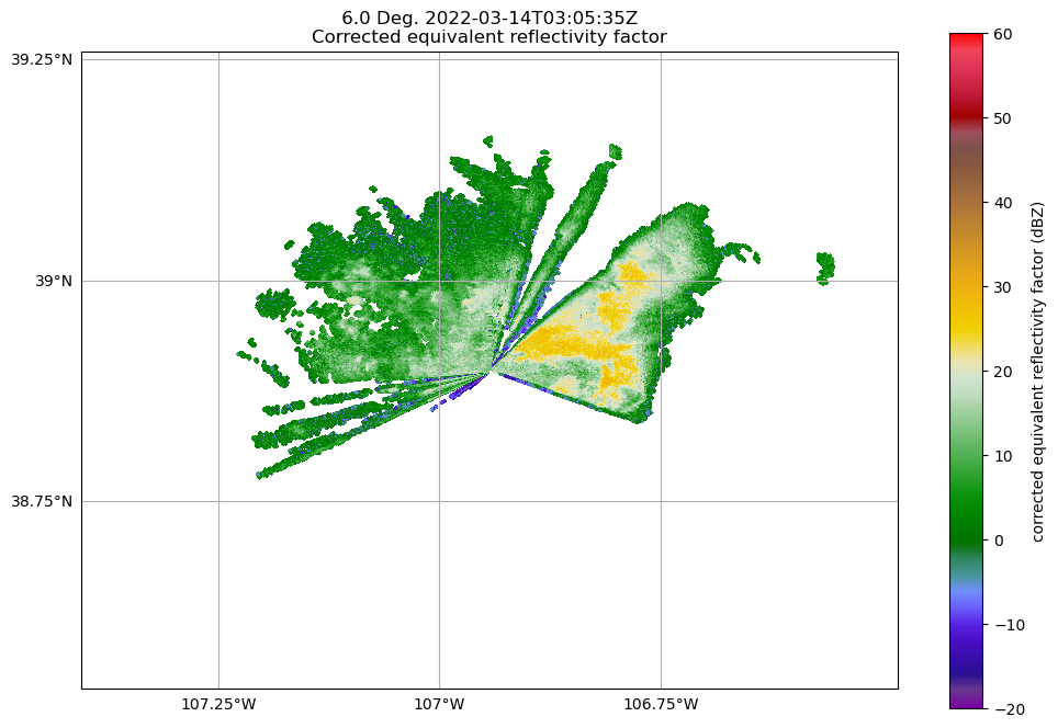
Or, let’s view a different elevation scan! To do this, change the sweep parameter in the plot_ppi_map function.
fig = plt.figure(figsize=[12, 8])
display = pyart.graph.RadarMapDisplay(radar)
display.plot_ppi_map('corrected_reflectivity',
                     sweep=6,
                     vmin=-20,
                     vmax=60,
                     lat_lines = np.arange(38, 39.5, .25),
                     lon_lines = np.arange(-107.5, -106.5, .25),
                     projection=ccrs.PlateCarree(),
                     cmap='pyart_Carbone42')
plt.show()
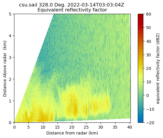
Plotting an RHI#
Another common plot that is requested by the radar community is a Range Height Indicator (RHI) Plot.
Fortunately, Py-ART has a utility to help us create one of these from our radar!
Read in an RHI file#
During this same time period during SAIL, the ARM program collected RHI scans, which provide a vertical cross section through the preciptiation! Let’s read in one of those files. The IO line is the same!
rhi_file = '../data/sample_sail_rhi.nc'
rhi_radar = pyart.io.read(rhi_file)
Plot our RHI#
We want to use the RadarDisplay here to visualize, using the reflectivity field (DBZ)
Note - this is uncorrected data, so be sure take caution working with this
radar = pyart.graph.RadarDisplay(rhi_radar)
radar.plot("DBZ", vmin=-20, vmax=60,)
plt.ylim(0, 5)
plt.savefig("sample-rhi.png", dpi=300)
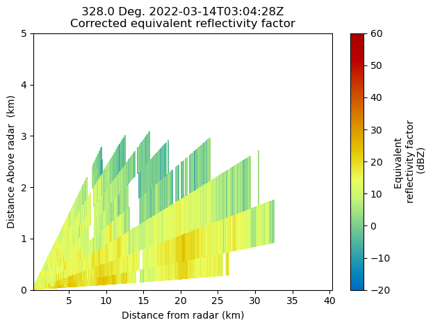
Add a “Pseudo-RHI” from our PPI data#
But let’s say we wanted to compare the vertical resolution we get from an RHI, compared to PPI… we can do this with Py-ART!
# Load our PPI data back in
file = '../data/sample_sail_ppi.nc'
radar = pyart.io.read(file)
radar

# Create a cross section at our 334 degree azimuth
xsect = pyart.util.cross_section_ppi(radar, [328])
Now, notice how coarse the resolution of the precipitation region!
colorbar_label = 'Equivalent \n reflectivity factor \n (dBZ)'
display = pyart.graph.RadarDisplay(xsect)
display.plot('corrected_reflectivity', 0, vmin=-20, vmax=60, colorbar_label=colorbar_label)
plt.ylim(0, 5)
plt.tight_layout()
Summary#
Within this notebook, we covered the basics of working with radar data using pyart, including:
Reading in a file using
pyart.ioInvestigating the
RadarobjectVisualizing radar data using the
RadarMapDisplay
What’s Next#
In the next few notebooks, we walk through gridding radar data, applying data cleaning methods, and advanced visualization methods!
Resources and References#
Py-ART essentials links: