Using EMC² to Process E3SM Output

Using EMC² to Process E3SM Output#

Overview of EMC²#

EMC² can be used to simulate radar and lidar observables faithful to large-scale model physics. Here, we will demonstrate using EMC² to evaluate a climate model’s output. We will process E3SM regional output around the fixed ARM site at Utqiagvik, North Slope of Alaska site, using EMC² radiation approach (fastest processing; faithful to E3SM’s radiation logic; similar general approach to that used for the on-line COSP).

We will briefly explore:#

Reading model output file using EMC²
Generating subcolumns and running the radar and lidar instrument simualtors
Classifying the simulator output
Plotting the simulated observables to evaluate the model output

Imports#

import emc2
import matplotlib as mpl
import numpy as np
import xarray as xr

Initializing Instrument Class Objects#

We begin with generating instrument class objects representing instruments deployed at Utqiagvik; that is, high spectral resolution lidar (HSRL) emc2.core.instruments.HSRL and ARM Ka-band Zenith Radar (KAZR) emc2.core.instruments.KAZR objects. Among other radar and lidar instruments, EMC² includes instrument sub-classes for the full ARM radar and lidar instrument suite. Note that in the case of the KAZR class object (as in the case of different radar object) we specify the ARM site string to initialize the KAZR class object with the correct radar attributes.

# Set instrument class objects to simulate (a radar and a lidar)
KAZR = emc2.core.instruments.KAZR('nsa')
HSRL = emc2.core.instruments.HSRL()
print("Instrument class generation done!")

Instrument class generation done!

Initializing a Model Class Object#

Let’s take a look at the model output data file from EAM (E3SM’s atmospheric component) using the xarray Python package.

Instead of explicitly using the xarray package to load the data, EMC² can automatically load the data file when generating an emc2.core.model.E3SM object. By using EMC² to load a large-scale model’s output, we are able to handle 2 potential issues exemplified in the examined E3SM output file:

Because E3SM operates a cube-sphere grid, data is not provided in a strict lat-lon grid (two spatial dimensions) but rather on a column basis (one spatial dimension). We need to inform EMC² about that by setting all_appended_in_lat=True.
The regional output file has appended strings at the end of every field name, the result of post-processing machinery. By setting appended_str=True, EMC² can remove these strings by using one of EMC²’s internal methods invoked during initialization.

Let’s generate an emc2.core.model.E3SM object and examine how the loaded data file is shown after initialization as an xr.Dataset object.

# Set model class object to use and load output file.
my_e3sm = emc2.core.model.E3SM(model_path, all_appended_in_lat=True, appended_str=True)
my_e3sm.ds  # shows the loaded dataset

./data/EMC2_demo_EAMv1_Freerun.2012-10-31.nc is a regional output dataset; Stacking the time, lat, and lon dims for processing with EMC^2.

<xarray.Dataset>
Dimensions:              (time_lat_lon: 72, lev: 72, cosp_prs: 7, nbnd: 2,
                          cosp_tau: 7, cosp_scol: 10, cosp_ht: 40, cosp_sr: 15,
                          cosp_sza: 5, cosp_htmisr: 16, cosp_tau_modis: 6,
                          ilev: 73, ncol_tmp: 3, time_tmp: 24)
Coordinates: (12/13)
  * time_lat_lon         (time_lat_lon) object (0, Timestamp('2012-10-31 01:0...
  * lev                  (lev) float64 998.5 993.8 986.2 ... 0.1828 0.1238
  * cosp_prs             (cosp_prs) float64 900.0 740.0 620.0 ... 245.0 90.0
  * cosp_tau             (cosp_tau) float64 0.15 0.8 2.45 6.5 16.2 41.5 219.5
  * cosp_scol            (cosp_scol) int32 1 2 3 4 5 6 7 8 9 10
  * cosp_ht              (cosp_ht) float64 240.0 720.0 ... 1.848e+04 1.896e+04
    ...                   ...
  * cosp_sza             (cosp_sza) float64 0.0 15.0 30.0 45.0 60.0
  * cosp_htmisr          (cosp_htmisr) float64 -99.0 0.25 0.75 ... 16.0 58.0
  * cosp_tau_modis       (cosp_tau_modis) float64 0.8 2.45 ... 41.5 5.003e+04
  * ilev                 (ilev) float64 0.1 0.1477 0.218 ... 990.5 997.0 1e+03
  * ncol_tmp             (ncol_tmp) int64 0 1 2
  * time_tmp             (time_tmp) datetime64[ns] 2012-10-31T01:00:00 ... 20...
Dimensions without coordinates: nbnd
Data variables: (12/209)
    lat                  (time_lat_lon) float64 dask.array<chunksize=(72,), meta=np.ndarray>
    lon                  (time_lat_lon) float64 dask.array<chunksize=(72,), meta=np.ndarray>
    cosp_prs_bnds        (cosp_prs, nbnd) float64 dask.array<chunksize=(7, 2), meta=np.ndarray>
    cosp_tau_bnds        (nbnd, cosp_tau) float64 dask.array<chunksize=(2, 7), meta=np.ndarray>
    cosp_ht_bnds         (nbnd, cosp_ht) float64 dask.array<chunksize=(2, 40), meta=np.ndarray>
    cosp_sr_bnds         (nbnd, cosp_sr) float64 dask.array<chunksize=(2, 15), meta=np.ndarray>
    ...                   ...
    wat_a2               (time_lat_lon, lev) float32 3.821e-12 4.221e-12 ... 0.0
    wat_a3               (time_lat_lon, lev) float32 2.606e-09 2.898e-09 ... 0.0
    wat_a4               (time_lat_lon, lev) float32 1.733e-17 1.919e-17 ... 0.0
    p_3d                 (time_lat_lon, lev) float64 dask.array<chunksize=(72, 72), meta=np.ndarray>
    zeros_cf             (time_lat_lon, lev) float64 0.0 0.0 0.0 ... 0.0 0.0 0.0
    rho_a                (time_lat_lon, lev) float64 dask.array<chunksize=(72, 72), meta=np.ndarray>
Attributes: (12/15)
    Conventions:          CF-1.0
    source:               CAM
    case:                 EAMv1_ARM_Freerun_1
    title:                UNSET
    logname:              yshi
    host:                 cori07
    ...                   ...
    topography_file:      /global/cfs/cdirs/e3sm/inputdata/atm/cam/topo/USGS-...
    time_period_freq:     hour_1
    _file_dates:          ['20121031']
    _file_times:          ['010000']
    _datastream:          act_datastream
    _arm_standards_flag:  0

Running the Subcolumn Generator and Instrument Simulator#

Now, we use the emc2.simulator.main.make_simulated_data method to have EMC² perform a set of (optional) tasks:

Generate user-specified number of subcolumns per model grid cell.
Run the instrument simualtor.
Classify hydrometeor phase using the simulated observables.

We first call the emc2.simulator.main.make_simulated_data method to calculate the HSRL observables and then call it again to calcualte the KAZR observables (without invoking the subcolumn generator methods again).

Note that because the model output contains the spatial dimension stacked onto the time dimension, we wish to unstack these dimensions once all simualtor operations are done by setting unstack_dims=True.

because the simulator is being run here using a 10-yr old machine, the processing timing printed on the screen is relatively longer than one should typically expect.

#Specify number of subcolumns and run simulator (first, for the lidar, then the radar) 
N_sub = 50
my_e3sm = emc2.simulator.main.make_simulated_data(my_e3sm, HSRL, N_sub, do_classify=True, convert_zeros_to_nan=True)
print("lidar processing done!")
my_model = emc2.simulator.main.make_simulated_data(my_e3sm, KAZR, N_sub, do_classify=True, convert_zeros_to_nan=True,
                                                   unstack_dims=True, skip_subcol_gen=True, finalize_fields=True)
print("radar processing done!")

## Creating subcolumns...
No convective processing for E3SM
Now performing parallel stratiform hydrometeor allocation in subcolumns
Fully overcast cl & ci in 649 voxels
Done! total processing time = 7.33s
Now performing parallel strat precipitation allocation in subcolumns
Fully overcast pl & pi in 420 voxels
Done! total processing time = 8.80s
Generating lidar moments...
Generating stratiform lidar variables using radiation logic
2-D interpolation of bulk liq lidar backscattering using mu-lambda values
2-D interpolation of bulk liq lidar extinction using mu-lambda values
Done! total processing time = 0.55s
'pl' not in hyd_types = ['cl', 'ci', 'pi']; excluding from COSP calculations
lidar processing done!
## Creating subcolumns...
Skipping subcolumn generator (make sure subcolumns were already generated).
Generating radar moments...
Generating stratiform radar variables using radiation logic
2-D interpolation of bulk liq radar backscattering using mu-lambda values
2-D interpolation of bulk liq radar extinction using mu-lambda values
Done! total processing time = 0.42s
Unstacking the time dimension (time, lat, and lon dimensions)
radar processing done!

We can examine the simulator output dataset saved under an `xr.Dataset` object. We can see that for most lidar and radar observables (the equivalent reflectivity factor Ze, the backscatter cross-section beta_p, etc.) we have fields per hydrometeor class in addition to the field representing the total.#

my_e3sm.ds

<xarray.Dataset>
Dimensions:                           (ncol: 3, time: 24, lev: 72,
                                       subcolumn: 50, ilev: 73, cosp_prs: 7,
                                       nbnd: 2, cosp_tau: 7, cosp_scol: 10,
                                       cosp_ht: 40, cosp_sr: 15, cosp_sza: 5,
                                       cosp_htmisr: 16, cosp_tau_modis: 6)
Coordinates: (12/13)
  * ncol                              (ncol) int64 0 1 2
  * time                              (time) datetime64[ns] 2012-10-31T01:00:...
  * lev                               (lev) float64 998.5 993.8 ... 0.1238
  * subcolumn                         (subcolumn) int64 0 1 2 3 ... 46 47 48 49
  * ilev                              (ilev) float64 0.1 0.1477 ... 997.0 1e+03
  * cosp_prs                          (cosp_prs) float64 900.0 740.0 ... 90.0
    ...                                ...
  * cosp_scol                         (cosp_scol) int32 1 2 3 4 5 6 7 8 9 10
  * cosp_ht                           (cosp_ht) float64 240.0 ... 1.896e+04
  * cosp_sr                           (cosp_sr) float64 0.605 2.1 ... 1.004e+03
  * cosp_sza                          (cosp_sza) float64 0.0 15.0 30.0 45.0 60.0
  * cosp_htmisr                       (cosp_htmisr) float64 -99.0 0.25 ... 58.0
  * cosp_tau_modis                    (cosp_tau_modis) float64 0.8 ... 5.003e+04
Dimensions without coordinates: nbnd
Data variables: (12/268)
    lat                               (time, ncol) float64 72.89 71.18 ... 70.44
    lon                               (time, ncol) float64 202.9 204.9 ... 203.8
    cosp_prs_bnds                     (cosp_prs, nbnd) float64 dask.array<chunksize=(7, 2), meta=np.ndarray>
    cosp_tau_bnds                     (nbnd, cosp_tau) float64 dask.array<chunksize=(2, 7), meta=np.ndarray>
    cosp_ht_bnds                      (nbnd, cosp_ht) float64 dask.array<chunksize=(2, 40), meta=np.ndarray>
    cosp_sr_bnds                      (nbnd, cosp_sr) float64 dask.array<chunksize=(2, 15), meta=np.ndarray>
    ...                                ...
    sub_col_Ze_att_tot_strat          (subcolumn, time, lev, ncol) float64 na...
    Ze_min                            (time, lev, ncol) float32 -87.04 ... -1...
    sub_col_Ze_tot                    (subcolumn, time, lev, ncol) float64 na...
    sub_col_Ze_att_tot                (subcolumn, time, lev, ncol) float64 na...
    detect_mask                       (subcolumn, time, lev, ncol) bool False...
    phase_mask_KAZR_sounding_all_hyd  (subcolumn, time, lev, ncol) float64 na...
Attributes: (12/15)
    Conventions:          CF-1.0
    source:               CAM
    case:                 EAMv1_ARM_Freerun_1
    title:                UNSET
    logname:              yshi
    host:                 cori07
    ...                   ...
    topography_file:      /global/cfs/cdirs/e3sm/inputdata/atm/cam/topo/USGS-...
    time_period_freq:     hour_1
    _file_dates:          ['20121031']
    _file_times:          ['010000']
    _datastream:          act_datastream
    _arm_standards_flag:  0

Visualization#

We can plot EMC² output using matplotlib, xarray’s internal methods, or EMC²’s emc2.plotting.SubcolumnDisplay object, which is based on the ACT package. Here, using the SubcolumnDisplay’s plot_subcolumn_timeseries method, we show the height x time curtain of the first subcolumn (out of the 50 specified) in the grid cell closest to the coordinates of the Utqiagvik specified using the lat_sel and lon_sel keywords. The hatch patterns invoked by setting hatched_mask=True, designate subcolumn bins not detected by the simulated instrument.

# set Matplotlib's shading parameter
mpl.rcParams['pcolor.shading'] = 'auto'

# Set input parameters.
cmap = 'viridis'
field_to_plot = ["sub_col_beta_p_tot", "sub_col_alpha_p_tot", "sub_col_OD_tot", "sub_col_Ze_att_tot"]
vmin_max = [(1e-8,1e-3), (1e-6, 1e-1), (0, 16), (-50., 10.)]
log_plot = [True, True, False, False]
is_radar_field = [False, False, False, True]
y_range = (200., 1e3)  # in hPa
subcol_ind = 0
NSA_coords = {"lat": 71.32, "lon": -156.61}

# Generate a SubcolumnDisplay object for coords closest to the NSA site
model_display = emc2.plotting.SubcolumnDisplay(my_e3sm, subplot_shape=(1, 4), figsize=(15,5),
                                               lat_sel=NSA_coords["lat"],
                                               lon_sel=NSA_coords["lon"], tight_layout=True)

# set intrument detectability masks for KAZR and HSRL
Mask_array_KAZR_model = model_display.model.ds["detect_mask"].isel(subcolumn=subcol_ind)
Mask_array_HSRL_model = model_display.model.ds["ext_mask"].isel(subcolumn=subcol_ind)

# Plot variables
for ii in range(4):
    if is_radar_field[ii]:
        Mask_array=Mask_array_KAZR_model
    else:
        Mask_array=Mask_array_HSRL_model
    model_display.plot_subcolumn_timeseries(field_to_plot[ii], subcol_ind, log_plot=log_plot[ii], y_range=y_range,
                                            subplot_index=(0, ii),  cmap=cmap, title='',
                                            vmin=vmin_max[ii][0], vmax=vmin_max[ii][1],
                                            Mask_array=Mask_array, hatched_mask=True)

cropping lat dim (lat requested = 71.32)

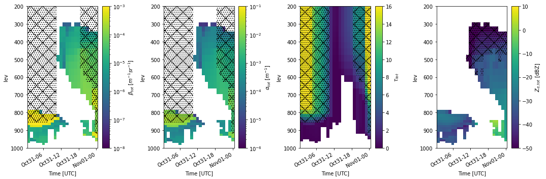
../../../_images/5ff2083aece7f78a90e46b4e0154686d85570434c8b0db67941aaa27d5e2881d.png

For a given subcolumn, we can also plot the output from one of the phase classification algorithms (HSRL-based classification in this case) by using the plot_subcolumn_timeseries method followed by calling the change_plot_to_class_mask.

Another option is to use the phase classification output and the emc2.simulator.classification.calculate_phase_ratio method to calcualte the hydrometeor phase partitioning based on all subcolumns, which we can then plot. Here, we also use the SubcolumnDisplay’s fig.savefig method to save the figure as a PNG file.

# Generate a SubcolumnDisplay object for coords closest to the NSA site
model_display2 = emc2.plotting.SubcolumnDisplay(my_e3sm, subplot_shape=(2, 1), figsize=(10,10),
                                               lat_sel=NSA_coords["lat"],
                                               lon_sel=NSA_coords["lon"], tight_layout=True)

# Plot classification mask output for a given subcolumn
_, cb2_1 = model_display2.plot_subcolumn_timeseries("phase_mask_HSRL_all_hyd", subcol_ind, y_range=y_range,
                                        subplot_index=(0),  title='')
model_display2.change_plot_to_class_mask(cb2_1, variable="phase_mask_HSRL_all_hyd", convert_zeros_to_nan=True)

# Calculate frequency phase ratio
my_e3sm = emc2.simulator.classification.calculate_phase_ratio(my_e3sm, "phase_mask_HSRL_all_hyd", [1])

# Plot frequency phase ratio based on simulated data from all subcolumns
model_display2.plot_subcolumn_timeseries("phase_mask_HSRL_all_hyd_fpr", subcol_ind, y_range=y_range,
                                         cmap="bwr", subplot_index=(1),
                                         cbar_label='Frequency pr (reddish - more liquid)')
model_display2.fig.savefig('HSRL_simulated_class.png', dpi=150)

cropping lat dim (lat requested = 71.32)

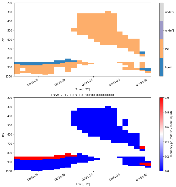
../../../_images/6596e9cbdba5b1e1cd1e818c5ded41cc6b83bc24df13b6139421df2011aafc27.png

Recalling that EMC² outputs radar and lidar observables per hydrometeor class, we can examine a breakdown of hydrometeor contribution to every simulated observable. This type of analysis also enables the evaluation of the classification algorithm, generally speaking. Note that because we examine variables per hydrometeor class, we ignore the detectability constraints here. Also note that the user can quite easily edit the “cosmetics” (fontsize, etc.) when calling the plotting method, but we skip these options in this example.

# Set additional input parameters.
field_to_plot_per_class = \
    ["sub_col_beta_p_%s_strat", "sub_col_alpha_p_%s_strat", "sub_col_OD_%s_strat", "sub_col_Ze_%s_strat"]
hyd_class = my_e3sm.hyd_types

# generate a SubcolumnDisplay object for coords closest to the NSA site.
model_display3 = emc2.plotting.SubcolumnDisplay(my_e3sm, subplot_shape=(len(hyd_class), 4), figsize=(15, 5 * len(hyd_class)),
                                               lat_sel=NSA_coords["lat"],
                                               lon_sel=NSA_coords["lon"], tight_layout=True)

# Plot variables per hydrometeor class
for ii in range(4):
    for class_i in range(len(hyd_class)):
        if is_radar_field[ii]:
            Mask_array=Mask_array_KAZR_model
        else:
            Mask_array=Mask_array_HSRL_model
        model_display3.plot_subcolumn_timeseries(field_to_plot_per_class[ii] % hyd_class[class_i], subcol_ind,
                                                log_plot=log_plot[ii], y_range=y_range,
                                                subplot_index=(class_i, ii),  cmap=cmap, title=hyd_class[class_i],
                                                vmin=vmin_max[ii][0], vmax=vmin_max[ii][1])

cropping lat dim (lat requested = 71.32)

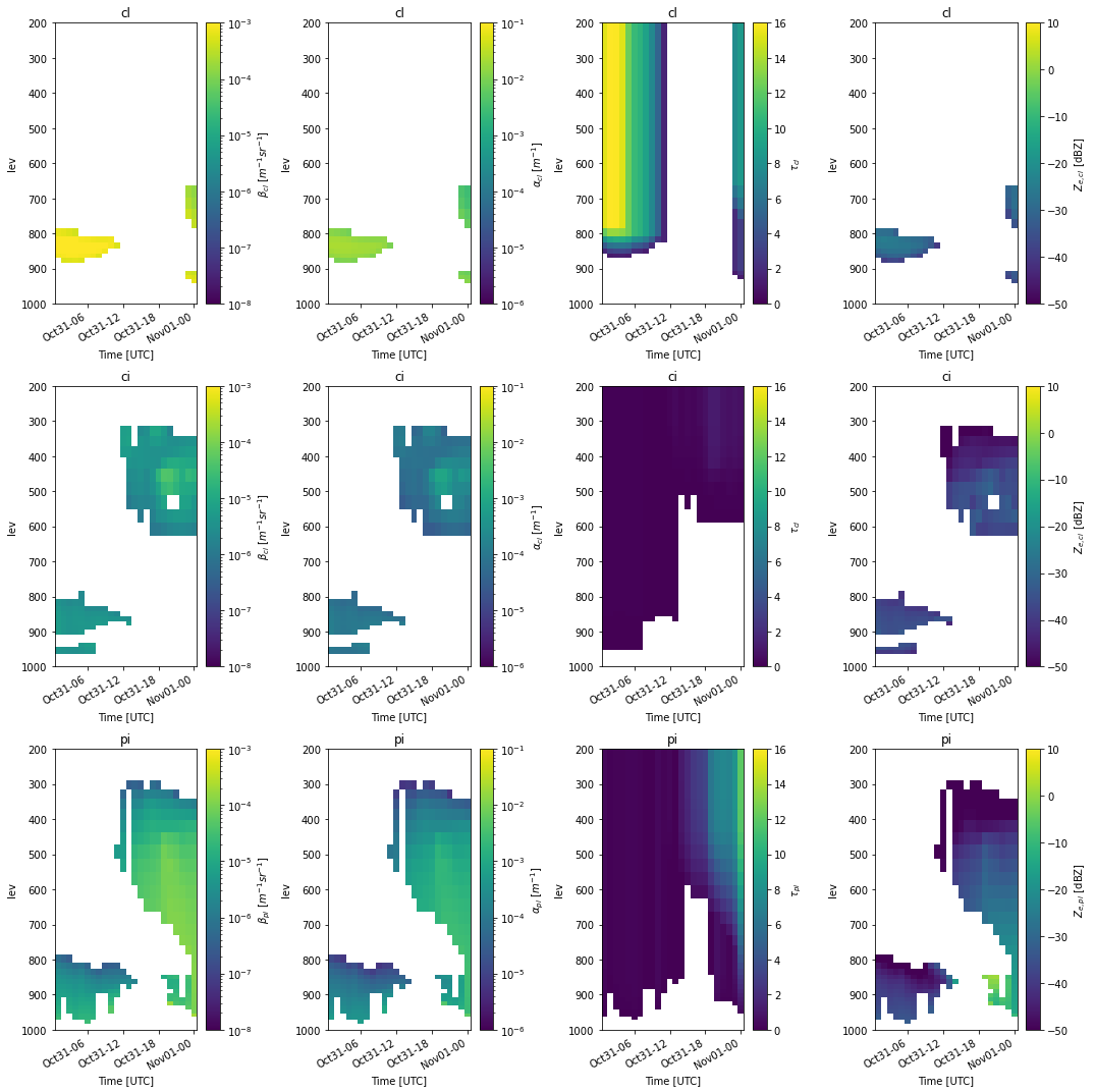
../../../_images/b10f8c45697c11eb75b8549711f27d09fb34225bfce414d4b91cad15fbf7485f.png

In addition to plotting the temporal evolution of a specific subcolun, we can also plot all subcolumns at a single time step using the SubcolumnDisplay’s plot_single_profile method.

# Specify time step to examine
Time = np.array('2012-10-31T21:00', dtype='datetime64')

# generate a SubcolumnDisplay object for coords closest to the NSA site.
model_display4 = emc2.plotting.SubcolumnDisplay(my_e3sm, subplot_shape=(1, 4), figsize=(15, 5),
                                               lat_sel=NSA_coords["lat"], lon_sel=NSA_coords["lon"],
                                               tight_layout=True)

# Plot variables at a given time step.
for ii in range(4):
    model_display4.plot_single_profile(field_to_plot[ii], time=Time, log_plot=log_plot[ii], y_range=y_range,
                                            subplot_index=(0, ii),  cmap=cmap, title=Time,
                                            vmin=vmin_max[ii][0], vmax=vmin_max[ii][1])

cropping lat dim (lat requested = 71.32)

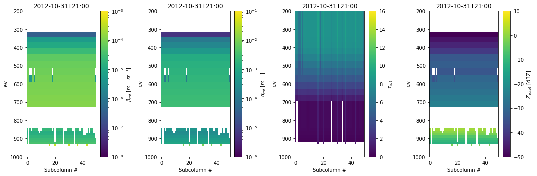
../../../_images/019ccc7fbfee4f686b3b41b146952c25cb7c164352fdbf56fb4e8c02a86e92d4.png

We can also examine mean profiles using the plot_subcolumn_mean_profile method. This method also illustrates the stardard deviation as an envelope around the mean. Note that here we plot the mean profile as a function of height instead of pressure coordinates by setting pressure_coords=False when invoking the plotting routine.

# Specify height range to plot (previously we plotted the pressure level on the y-axis)
y_range_h = (0., 12000)

# generate a SubcolumnDisplay object for coords closest to the NSA site
model_display5 = emc2.plotting.SubcolumnDisplay(my_e3sm, subplot_shape=(1, 4), figsize=(15, 5),
                                               lat_sel=NSA_coords["lat"], lon_sel=NSA_coords["lon"],
                                               tight_layout=True)

# Plot variable mean profiles
for ii in range(4):
    model_display5.plot_subcolumn_mean_profile(field_to_plot[ii], time=Time, log_plot=log_plot[ii], y_range=y_range_h,
                                              subplot_index=(0, ii),  title=Time, pressure_coords=False,
                                              x_range=vmin_max[ii])

cropping lat dim (lat requested = 71.32)

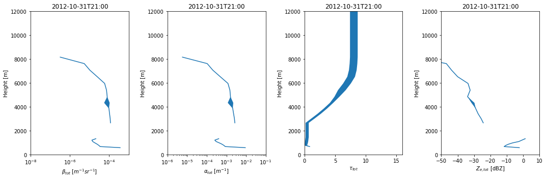
../../../_images/afd749b8ee1e9a83c69d7bcc7c0ff75f8c2ab23464a31d90d5b334d0a28e5955.png

Concluding Remarks#

EMC² includes support for a large number of instruments including the full ARM radar and lidar instrument suite and has already been operated on ESM, SCM, and LES outputs. The software include multiple methods for phase classification and partitioning, scattering calculations, and more. See and follow the continuously updated EMC² GitHub repository for more information.