
Py-ART Gridding#
Overview#
Within this notebook, we will cover:
What is gridding and why is it important?
An overview of gridding with Py-ART
How to choose a gridding routine
Gridding multiple radars to the same grid
Prerequisites#
Concepts |
Importance |
Notes |
|---|---|---|
Helpful |
Basic features |
|
Helpful |
Basic features |
|
Helpful |
Basic plotting |
|
Helpful |
Basic arrays |
Time to learn: 45 minutes
Imports#
import os
import warnings

import cartopy.crs as ccrs
import matplotlib.pyplot as plt


import pyart

warnings.filterwarnings('ignore')
## You are using the Python ARM Radar Toolkit (Py-ART), an open source
## library for working with weather radar data. Py-ART is partly
## supported by the U.S. Department of Energy as part of the Atmospheric
## Radiation Measurement (ARM) Climate Research Facility, an Office of
## Science user facility.
##
## If you use this software to prepare a publication, please cite:
##
##     JJ Helmus and SM Collis, JORS 2016, doi: 10.5334/jors.119
<frozen importlib._bootstrap>:283: DeprecationWarning: the load_module() method is deprecated and slated for removal in Python 3.12; use exec_module() instead
/Users/mgrover/miniforge3/envs/pyart-docs/lib/python3.10/site-packages/tqdm/auto.py:22: TqdmWarning: IProgress not found. Please update jupyter and ipywidgets. See https://ipywidgets.readthedocs.io/en/stable/user_install.html
  from .autonotebook import tqdm as notebook_tqdm
What is gridding and why is it important?#
Antenna vs. Cartesian Coordinates#
Radar data, by default, is stored in a polar (or antenna) coordinate system, with the data coordinates stored as an angle (ranging from 0 to 360 degrees with 0 == North), and a radius from the radar, and an elevation which is the angle between the ground and the ground.
This format can be challenging to plot, since it is scan/radar specific. Also, it can make comparing with model data, which is on a lat/lon grid, challenging since one would need to transform the model daa cartesian coordinates to polar/antenna coordiantes.
Fortunately, PyART has a variety of gridding routines, which can be used to grid your data to a Cartesian grid. Once it is in this new grid, one can easily slice/dice the dataset, and compare to other data sources.
Why is Gridding Important?#
Gridding is essential to combining multiple data sources (ex. multiple radars), and comparing to other data sources (ex. model data). There are also decisions that are made during the gridding process that have a large impact on the regridded data - for example:
What resolution should my grid be?
Which interpolation routine should I use?
How smooth should my interpolated data be?
While there is not always a right or wrong answer, it is important to understand the options available, and document which routine you used with your data! Also - experiment with different options and choose the best for your use case!
An overview of gridding with Py-ART#
Let’s dig into the regridding process with PyART!
Read in and Visualize a Test Dataset#
Let’s start with the same file used in the previous notebook (PyART Basics), which is a radar file from Northern Oklahoma.
file = "../data/sample_sail_ppi.nc"
radar = pyart.io.read(file)
Let’s plot up quick look of reflectivity, at the lowest elevation scan (closest to the ground)
fig = plt.figure(figsize=[12, 12])
display = pyart.graph.RadarDisplay(radar)
display.plot_ppi('corrected_reflectivity',
                 3,
                 cmap='pyart_HomeyerRainbow')
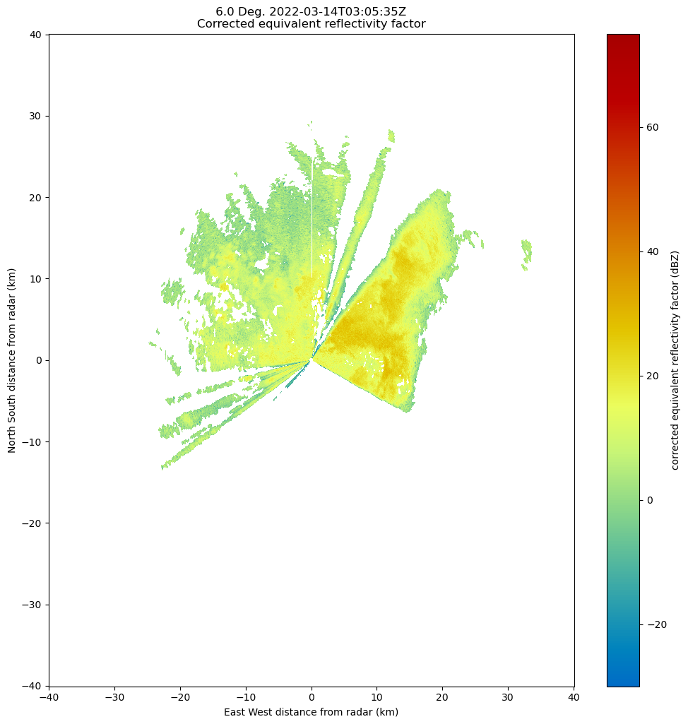
As mentioned before, the dataset is currently in the antenna coordinate system measured as distance from the radar
Setup our Gridding Routine with pyart.map.grid_from_radars()#
Py-ART has the Grid object which has characteristics similar to that of the Radar object, except that the data are stored in Cartesian coordinates instead of the radar’s antenna coordinates.
pyart.core.Grid?
Init signature:
pyart.core.Grid(
    time,
    fields,
    metadata,
    origin_latitude,
    origin_longitude,
    origin_altitude,
    x,
    y,
    z,
    projection=None,
    radar_latitude=None,
    radar_longitude=None,
    radar_altitude=None,
    radar_time=None,
    radar_name=None,
)
Docstring:
A class for storing rectilinear gridded radar data in Cartesian coordinate.

Refer to the attribute section for information on the parameters.

To create a Grid object using legacy parameters present in Py-ART version
1.5 and before, use :py:func:`from_legacy_parameters`,
grid = Grid.from_legacy_parameters(fields, axes, metadata).

Attributes
----------
time : dict
    Time of the grid.
fields : dict of dicts
    Moments from radars or other variables.
metadata : dict
    Metadata describing the grid.
origin_longitude, origin_latitude, origin_altitude : dict
    Geographic coordinate of the origin of the grid.
x, y, z : dict, 1D
    Distance from the grid origin for each Cartesian coordinate axis in a
    one dimensional array. Defines the spacing along the three grid axes
    which is repeated throughout the grid, making a rectilinear grid.
nx, ny, nz : int
    Number of grid points along the given Cartesian dimension.
projection : dic or str
    Projection parameters defining the map projection used to transform
    from Cartesian to geographic coordinates. None will use the default
    dictionary with the 'proj' key set to 'pyart_aeqd' indicating that
    the native Py-ART azimuthal equidistant projection is used. Other
    values should specify a valid pyproj.Proj projparams dictionary or
    string. The special key '_include_lon_0_lat_0' is removed when
    interpreting this dictionary. If this key is present and set to True,
    which is required when proj='pyart_aeqd', then the radar longitude and
    latitude will be added to the dictionary as 'lon_0' and 'lat_0'.
    Use the :py:func:`get_projparams` method to retrieve a copy of this
    attribute dictionary with this special key evaluated.
radar_longitude, radar_latitude, radar_altitude : dict or None, optional
    Geographic location of the radars which make up the grid.
radar_time : dict or None, optional
    Start of collection for the radar which make up the grid.
radar_name : dict or None, optional
    Names of the radars which make up the grid.
nradar : int
    Number of radars whose data was used to make the grid.
projection_proj : Proj
    pyproj.Proj instance for the projection specified by the projection
    attribute. If the 'pyart_aeqd' projection is specified accessing this
    attribute will raise a ValueError.
point_x, point_y, point_z : LazyLoadDict
    The Cartesian locations of all grid points from the origin in the
    three Cartesian coordinates. The three dimensional data arrays
    contained these attributes are calculated from the x, y, and z
    attributes. If these attributes are changed use :py:func:
    `init_point_x_y_z` to reset the attributes.
point_longitude, point_latitude : LazyLoadDict
    Geographic location of each grid point. The projection parameter(s)
    defined in the `projection` attribute are used to perform an inverse
    map projection from the Cartesian grid point locations relative to
    the grid origin. If these attributes are changed use
    :py:func:`init_point_longitude_latitude` to reset the attributes.
point_altitude : LazyLoadDict
    The altitude of each grid point as calculated from the altitude of the
    grid origin and the Cartesian z location of each grid point.  If this
    attribute is changed use :py:func:`init_point_altitude` to reset the
    attribute.
Init docstring: Initalize object.
File:           ~/git_repos/pyart/pyart/core/grid.py
Type:           type
Subclasses:
We can transform our data into this grid object, from the radars, using pyart.map.grid_from_radars().
Beforing gridding our data, we need to make a decision about the desired grid resolution and extent. For example, one might imagine a grid configuration of:
Grid extent/limits
20 km in the x-direction (north/south)
20 km in the y-direction (west/east)
15 km in the z-direction (vertical)
500 m spatial resolution
The pyart.map.grid_from_radars() function takes the grid shape and grid limits as input, with the order (z, y, x).
Let’s setup our configuration, setting our grid extent first, with the distance measured in meters
z_grid_limits = (500.,15_000.)
y_grid_limits = (-20_000.,20_000.)
x_grid_limits = (-20_000.,20_000.)
Now that we have our grid limits, we can set our desired resolution (again, in meters)
grid_resolution = 500
Let’s compute our grid shape - using the extent and resolution to compute the number of grid points in each direction.
def compute_number_of_points(extent, resolution):
    return int((extent[1] - extent[0])/resolution)
Now that we have a helper function to compute this, let’s apply it to our vertical dimension
z_grid_points = compute_number_of_points(z_grid_limits, grid_resolution)
z_grid_points
29
We can apply this to the horizontal (x, y) dimensions as well.
x_grid_points = compute_number_of_points(x_grid_limits, grid_resolution)
y_grid_points = compute_number_of_points(y_grid_limits, grid_resolution)

print(z_grid_points,
      y_grid_points,
      x_grid_points)
29 80 80
Use our configuration to grid the data!#
Now that we have the grid shape and grid limits, let’s grid up our radar!
grid = pyart.map.grid_from_radars(radar,
                                  grid_shape=(z_grid_points,
                                              y_grid_points,
                                              x_grid_points),
                                  grid_limits=(z_grid_limits,
                                               y_grid_limits,
                                               x_grid_limits),
                                 )
grid
<pyart.core.grid.Grid at 0x1667fc580>
We now have a pyart.core.Grid object!
Plot up the Grid Object#
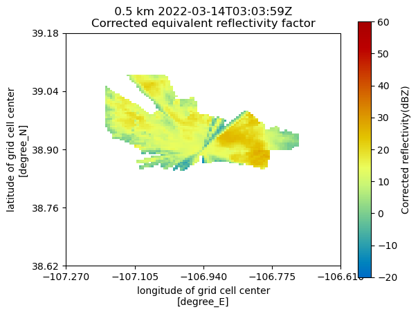
Plot a horizontal view of the data#
We can use the GridMapDisplay from pyart.graph to visualize our regridded data, starting with a horizontal view (slice along a single vertical level)
display = pyart.graph.GridMapDisplay(grid)
display.plot_grid('corrected_reflectivity',
                  level=0,
                  vmin=-20,
                  vmax=60,
                  cmap='pyart_HomeyerRainbow')
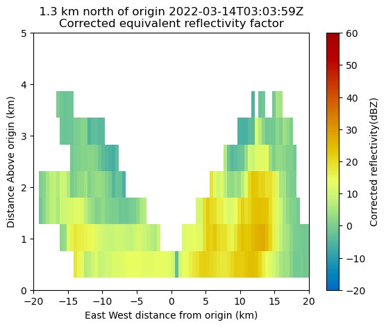
Plot a Latitudinal Slice#
We can also slice through a single latitude or longitude!
display.plot_latitude_slice('corrected_reflectivity',
                            lat=38.91,
                            vmin=-20,
                            vmax=60,
                            cmap='pyart_HomeyerRainbow')
plt.xlim([-20, 20])
plt.ylim([0, 5])
(0.0, 5.0)
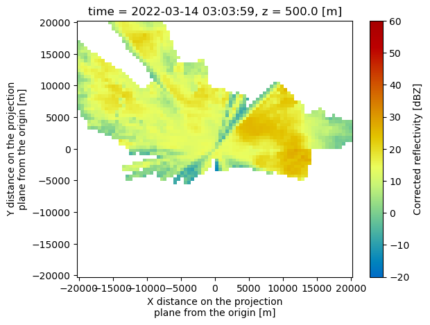
Plot with Xarray#
Another neat feature of the Grid object is that we can transform it to an xarray.Dataset!
ds = grid.to_xarray()
ds
<xarray.Dataset>
Dimensions:                              (time: 1, z: 29, y: 80, x: 80)
Coordinates:
  * time                                 (time) object 2022-03-14 03:03:59
  * z                                    (z) float64 500.0 1.018e+03 ... 1.5e+04
    lat                                  (y) float64 38.72 38.72 ... 39.07 39.08
    lon                                  (x) float64 -107.2 -107.2 ... -106.7
  * y                                    (y) float64 -2e+04 -1.949e+04 ... 2e+04
  * x                                    (x) float64 -2e+04 -1.949e+04 ... 2e+04
Data variables:
    corrected_differential_phase         (time, z, y, x) float64 0.01 ... nan
    corrected_reflectivity               (time, z, y, x) float64 nan nan ... nan
    corrected_velocity                   (time, z, y, x) float64 nan nan ... nan
    corrected_differential_reflectivity  (time, z, y, x) float64 nan nan ... nan
    corrected_specific_diff_phase        (time, z, y, x) float64 0.0 0.0 ... nan
ROI (time, z, y, x) float32 765.6 ... 1....Now, our plotting routine is a one-liner, starting with the horizontal slice:
ds.isel(z=0).corrected_reflectivity.plot(cmap='pyart_HomeyerRainbow',
                                         vmin=-20,
                                         vmax=60);
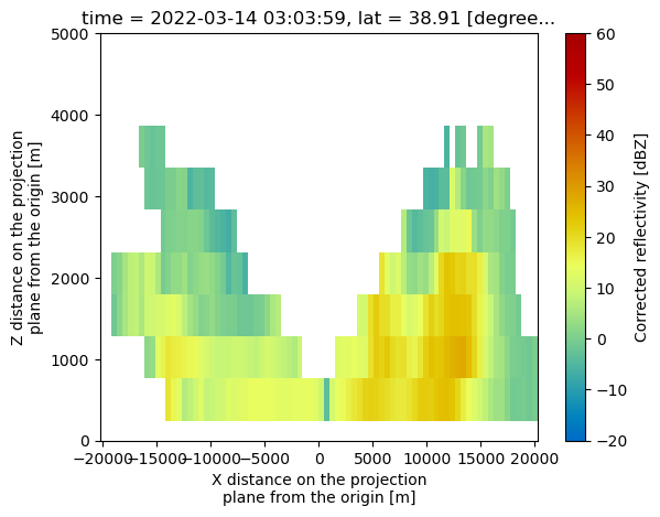
And a vertical slice at a given y dimension (latitude)
ds.sel(y=1300,
       method='nearest').corrected_reflectivity.plot(cmap='pyart_HomeyerRainbow',
                                                     vmin=-20,
                                                     vmax=60)
plt.ylim([0, 5000])
(0.0, 5000.0)
Summary#
Within this notebook, we covered the basics of gridding radar data using pyart, including:
What we mean by gridding and why is it matters
Configuring your gridding routine
Visualize gridded radar data
What’s Next#
In the next few notebooks, we walk through applying data cleaning methods, and advanced visualization methods!
Resources and References#
Py-ART essentials links: