Py-ART Basics with Xradar¶

Overview¶

History of the Python ARM Radar Toolkit (Py-ART)¶

Development began to address the needs of ARM with the acquisition of a number of new scanning cloud and precipitation radars as part of the American Recovery Act.
The project has since expanded to work with a variety of weather radars and a wider user base including radar researchers and climate modelers.
The software has been released on GitHub as open source software under a BSD license. Runs on Linux, OS X. It also runs on Windows with more limited functionality.

What can Py-ART Do?¶

Py-ART can be used for a variety of tasks from basic plotting to more complex processing pipelines (Helmus & Collis (2016)). Specific uses for Py-ART include:

pyart.io Module for reading radar data in a variety of file formats.
pyart.graph Module for creating plots and visualization of radar data.
pyart.correct Module for correcting radar moments while in antenna coordinates, such as:
- Doppler unfolding/de-aliasing.
- Attenuation correction.
- Phase processing using a Linear Programming method.
pyart.map Mapping data from one or multiple radars onto a Cartesian grid.
pyart.retrieve Performing retrievals.
pyart.io.write_cfradial Writing radial and Cartesian data to NetCDF files.

Py-ART 2.0¶

Py-ART 2.0 offers the option to use xradar for reading weather radar data into the xarray data model (Grover et al. (2026)). Py-ART 2.0 also supports cmweather, a new package dedicated to supporting color vision deficiency (CVD) friendly colormaps (Sherman et al. (2024)). Please check the linked documentation to view all the changes within Py-ART 2.0.

Prerequisites¶

Concepts	Importance	Notes
Intro to Cartopy	Helpful	Basic features
Weather Radar Basics	Helpful	Background Information
Matplotlib Basics	Helpful	Basic plotting
NumPy Basics	Helpful	Basic arrays
Xarray Basics	Helpful	Multi-dimensional arrays

Time to learn: 45 minutes

This tutorial will provide an introduction to Py-ART using the 23 April 2026 Enid, Oklahoma Enhanced Fujita (EF) Scale (EF-4) tornado outbreak, that passed near the X-Band ARM Scanning Preciptiation Radar (XSAPR) (Bharadwaj et al. (2026)) through:

Reading Data using Py-ART and xradar
Plotting the Radar Data
Gridding the Radar Data

# Uncomment if running on CoLab
##!pip install arm_pyart>=2.2.0
##!pip install xradar>=0.12.0

# Uncomment if running on CoLab
##import pathlib
##from pathlib import Path
##import gdown

##DATA_LINK = "1QLRRZMJ-HRQpbhATPqLfF8byJmnYWXzv"
##CREATE_BASE = pathlib.Path("../data")
##CREATE_BASE.mkdir(parents=True, exist_ok=True)
##gdown.download(id=DATA_LINK, output=str(CREATE_BASE / "sgpxsaprcfrI6.a1.20260423.233233.nc"), quiet=False)

Imports¶

import os
import warnings
import pathlib
from pathlib import Path

import cartopy.crs as ccrs
import matplotlib.pyplot as plt


import pyart
from pyart.testing import get_test_data
import xradar as xd
import cmweather

warnings.filterwarnings("ignore")


## You are using the Python ARM Radar Toolkit (Py-ART), an open source
## library for working with weather radar data. Py-ART is partly
## supported by the U.S. Department of Energy as part of the Atmospheric
## Radiation Measurement (ARM) Climate Research Facility, an Office of
## Science user facility.
##
## If you use this software to prepare a publication, please cite:
##
##     JJ Helmus and SM Collis, JORS 2016, doi: 10.5334/jors.119

Reading in Data Using Py-ART and xradar¶

Reading data in using `xradar.io.open_`¶

When reading in a radar file, we use the xradar.io module.

xradar.io can read a variety of different radar formats, such as Cf/Radial, ODIM_H5, etc. The documentation on what formats can be read by xradar can be found here:

xradar readers Documentation

Let’s take a look at one of these readers:

?xd.io.open_cfradial1_datatree

Signature: xd.io.open_cfradial1_datatree(filename_or_obj, **kwargs)
Docstring:
Open CfRadial1 dataset as :py:class:`xarray.DataTree`.

Parameters
----------
filename_or_obj : str, Path, file-like or xarray.DataStore
    Strings and Path objects are interpreted as a path to a local or remote
    radar file

Keyword Arguments
-----------------
sweep : int, list of int, optional
    Sweep number(s) to extract, default to first sweep. If None, all sweeps are
    extracted into a list.
first_dim : str
    Can be ``time`` or ``auto`` first dimension. If set to ``auto``,
    first dimension will be either ``azimuth`` or ``elevation`` depending on
    type of sweep. Defaults to ``auto``.
reindex_angle : bool or dict
    Defaults to False, no reindexing. Given dict should contain the kwargs to
    reindex_angle. Only invoked if `decode_coord=True`.
fix_second_angle : bool
    If True, fixes erroneous second angle data. Defaults to ``False``.
optional : bool
    Import optional mandatory data and metadata, defaults to ``True``.
site_as_coords : bool
    Attach radar site-coordinates to Dataset, defaults to ``True``.
engine: str
    Engine that will be passed to Xarray.open_dataset, defaults to "netcdf4"

Returns
-------
dtree: xarray.DataTree
    DataTree with CfRadial2 groups.
File:      ~/.vscode-micromamba/envs/arm-summer-school-2026-dev/lib/python3.11/site-packages/xradar/io/backends/cfradial1.py
Type:      function

Let’s use a sample data file from pyart - which is cfradial format.

When we read this in, we get a xarray.DataTree object that bundles the different radar sweeps into one structure!

# Where the pre-processed data lives.
# By default, we look within the repo's data folder/directory.
# If you've stored the files elsewhere, point save_dir at that directory, e.g. Path('/data/swe').
base_path = "../data/"
file = "sgpxsaprcfrI6.a1.20260423.233233.nc"
dt = xd.io.open_cfradial1_datatree(base_path + file)
dt

Investigate the `xradar` object¶

Within this xradar object object are the actual data fields, each stored in a different group, mimicking the FM301/cfradial2 data standard.

This is where data such as reflectivity and velocity are stored.

To see what fields are present we can add the fields and keys additions to the variable where the radar object is stored.

dt["sweep_0"]

Extract a sample data field¶

The fields are stored in a dictionary, each containing coordinates, units and more. All can be accessed by just adding the fields addition to the radar object variable.

For an individual field, we add a string in brackets after the fields addition to see the contents of that field.

Let’s take a look at 'corrected_reflectivity_horizontal', which is a common field to investigate.

print(dt["sweep_0"]["reflectivity"])

<xarray.DataArray 'reflectivity' (azimuth: 360, range: 1001)> Size: 1MB
[360360 values with dtype=float32]
Coordinates:
  * azimuth    (azimuth) float32 1kB 0.173 1.137 2.159 ... 357.2 358.1 359.2
    time       (azimuth) datetime64[ns] 3kB 2026-04-23T00:00:15.154999 ... 20...
    elevation  (azimuth) float32 1kB ...
  * range      (range) float32 4kB 0.0 100.0 200.0 ... 9.98e+04 9.99e+04 1e+05
Attributes:
    long_name:      Equivalent reflectivity factor
    units:          dBZ
    standard_name:  equivalent_reflectivity_factor

We can go even further in the dictionary and access the actual reflectivity data.

We use add .data at the end, which will extract the data array (which is a numpy array) from the dictionary.

reflectivity = dt["sweep_0"]["reflectivity"].data
print(type(reflectivity), reflectivity)

<class 'numpy.ndarray'> [[-50.14995      7.309805    -1.7119522  ...          nan   5.8390026
    0.31825733]
 [-49.818913     5.258644    -0.23067474 ...   2.0698109    1.4286919
    1.2987919 ]
 [-50.017952     6.3690786   -0.87179327 ...   8.09968      3.1886263
    0.29940128]
 ...
 [-49.68901      6.8593454   -0.49047422 ...   4.5190525   -0.33124208
    2.777975  ]
 [-49.39988      5.9290943   -0.8508415  ...          nan   3.4693775
           nan]
 [-50.229565     7.328661    -1.8711843  ...          nan  -3.3817945
    2.1997108 ]]

Lets’ check the size of this array...

reflectivity.shape

(360, 1001)

This reflectivity data array, numpy array, is a two-dimensional array with dimensions:

Range (distance away from the radar)
Azimuth (direction around the radar)

dt["sweep_0"].dims

Frozen(ChainMap({'azimuth': 360, 'range': 1001}, {'sweep': 18, 'frequency': 1}))

If we wanted to look the 300th ray, at the second gate, we would use something like the following:

print(reflectivity[300, 2])

1.969243

We can also select a specific azimuth if desired, using the xarray syntax:

# Since xradar is built upon xaray, we can use xarray's built in indexing and selection methods
dt["sweep_0"].sel(azimuth=180, method="nearest")

Plotting our Radar Data¶

An Overview of Py-ART Plotting Utilities¶

Now that we have loaded the data and inspected it, the next logical thing to do is to visualize the data! Py-ART’s visualization functionality is done through the objects in the pyart.graph module.

In Py-ART there are 4 primary visualization classes in pyart.graph:

Plotting grid data

GridMapDisplay

Use the RadarMapDisplay with our data¶

For the this example, we will be using RadarMapDisplay, using Cartopy to deal with geographic coordinates.

We start by creating a figure first, and adding our traditional radar methods to the xradar object.

fig = plt.figure(figsize=[10, 10])
radar = pyart.xradar.Xradar(dt)

<Figure size 1000x1000 with 0 Axes>

Once we have a figure, let’s add our RadarMapDisplay

fig = plt.figure(figsize=[10, 10])
display = pyart.graph.RadarMapDisplay(radar)

<Figure size 1000x1000 with 0 Axes>

Adding our map display without specifying a field to plot won’t do anything we need to specifically add a field to field using .plot_ppi_map()

display.plot_ppi_map("reflectivity")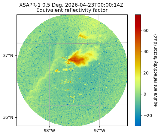

By default, it will plot the elevation scan, the the default colormap from Matplotlib... let’s customize!

We add the following arguements:

sweep=3 - The fourth elevation scan (since we are using Python indexing)
vmin=-20 - Minimum value for our plotted field/colorbar
vmax=60 - Maximum value for our plotted field/colorbar
projection=ccrs.PlateCarree() - Cartopy latitude/longitude coordinate system
cmap='pyart_HomeyerRainbow' - Colormap to use, selecting one provided by PyART

fig = plt.figure(figsize=[12, 12])
display = pyart.graph.RadarMapDisplay(radar)
display.plot_ppi_map(
    "reflectivity",
    sweep=3,
    vmin=-20,
    vmax=60,
    projection=ccrs.PlateCarree(),
    cmap="HomeyerRainbow",
)
plt.show()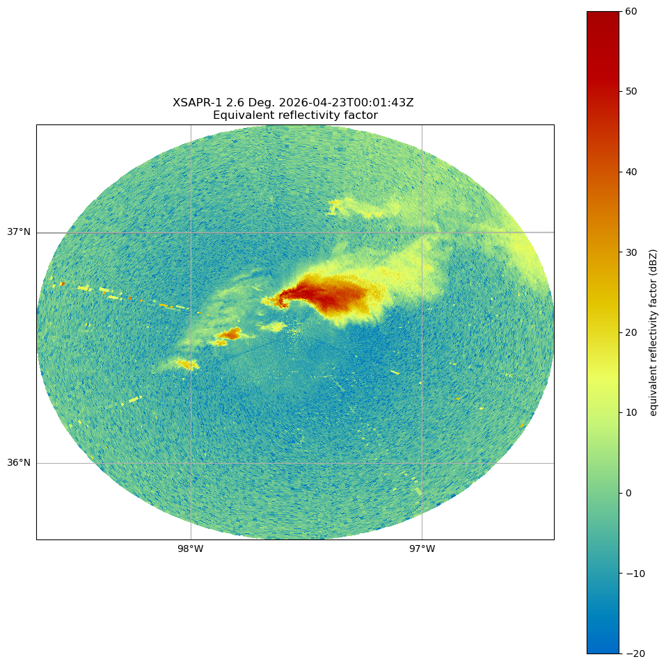

You can change many parameters in the graph by changing the arguments to plot_ppi_map. As you can recall from earlier. simply view these arguments in a Jupyter notebook by typing:

?display.plot_ppi_map

Signature:
display.plot_ppi_map(
    field,
    sweep=0,
    mask_tuple=None,
    vmin=None,
    vmax=None,
    cmap=None,
    norm=None,
    mask_outside=False,
    title=None,
    title_flag=True,
    colorbar_flag=True,
    colorbar_label=None,
    colorbar_orient='vertical',
    ax=None,
    fig=None,
    lat_lines=None,
    lon_lines=None,
    projection=None,
    min_lon=None,
    max_lon=None,
    min_lat=None,
    max_lat=None,
    width=None,
    height=None,
    lon_0=None,
    lat_0=None,
    resolution='110m',
    shapefile=None,
    shapefile_kwargs=None,
    edges=True,
    gatefilter=None,
    filter_transitions=True,
    embellish=True,
    add_grid_lines=True,
    raster=False,
    ticks=None,
    ticklabs=None,
    alpha=None,
    edgecolors='face',
    **kwargs,
)
Docstring:
Plot a PPI volume sweep onto a geographic map.

Parameters
----------
field : str
    Field to plot.
sweep : int, optional
    Sweep number to plot.

Other Parameters
----------------
mask_tuple : (str, float)
    Tuple containing the field name and value below which to mask
    field prior to plotting, for example to mask all data where
    NCP < 0.5 set mask_tuple to ['NCP', 0.5]. None performs no masking.
vmin : float
    Luminance minimum value, None for default value.
    Parameter is ignored is norm is not None.
vmax : float
    Luminance maximum value, None for default value.
    Parameter is ignored is norm is not None.
norm : Normalize or None, optional
    matplotlib Normalize instance used to scale luminance data. If not
    None the vmax and vmin parameters are ignored. If None, vmin and
    vmax are used for luminance scaling.
cmap : str or None
    Matplotlib colormap name. None will use the default colormap for
    the field being plotted as specified by the Py-ART configuration.
mask_outside : bool
    True to mask data outside of vmin, vmax. False performs no
    masking.
title : str
    Title to label plot with, None to use default title generated from
    the field and tilt parameters. Parameter is ignored if title_flag
    is False.
title_flag : bool
    True to add a title to the plot, False does not add a title.
colorbar_flag : bool
    True to add a colorbar with label to the axis. False leaves off
    the colorbar.
ticks : array
    Colorbar custom tick label locations.
ticklabs : array
    Colorbar custom tick labels.
colorbar_label : str
    Colorbar label, None will use a default label generated from the
    field information.
colorbar_orient : 'vertical' or 'horizontal'
    Colorbar orientation.
ax : Cartopy GeoAxes instance
    If None, create GeoAxes instance using other keyword info.
    If provided, ax must have a Cartopy crs projection and projection
    kwarg below is ignored.
fig : Figure
    Figure to add the colorbar to. None will use the current figure.
lat_lines, lon_lines : array or None
    Locations at which to draw latitude and longitude lines.
    None will use default values which are resonable for maps of
    North America.
projection : cartopy.crs class
    Map projection supported by cartopy. Used for all subsequent calls
    to the GeoAxes object generated. Defaults to LambertConformal
    centered on radar.
min_lat, max_lat, min_lon, max_lon : float
    Latitude and longitude ranges for the map projection region in
    degrees.
width, height : float
    Width and height of map domain in meters.
    Only this set of parameters or the previous set of parameters
    (min_lat, max_lat, min_lon, max_lon) should be specified.
    If neither set is specified then the map domain will be determined
    from the extend of the radar gate locations.
shapefile : str
    Filename for a shapefile to add to map.
shapefile_kwargs : dict
    Key word arguments used to format shapefile. Projection defaults
    to lat lon (cartopy.crs.PlateCarree())
resolution : '10m', '50m', '110m'.
    Resolution of NaturalEarthFeatures to use. See Cartopy
    documentation for details.
gatefilter : GateFilter
    GateFilter instance. None will result in no gatefilter mask being
    applied to data.
filter_transitions : bool
    True to remove rays where the antenna was in transition between
    sweeps from the plot. False will include these rays in the plot.
    No rays are filtered when the antenna_transition attribute of the
    underlying radar is not present.
edges : bool
    True will interpolate and extrapolate the gate edges from the
    range, azimuth and elevations in the radar, treating these
    as specifying the center of each gate. False treats these
    coordinates themselved as the gate edges, resulting in a plot
    in which the last gate in each ray and the entire last ray are not
    not plotted.
embellish: bool
    True by default. Set to False to supress drawing of coastlines
    etc.. Use for speedup when specifying shapefiles.
add_grid_lines : bool
    True by default. Set to False to supress drawing of lat/lon lines
    Note that lat lon labels only work with certain projections.
raster : bool
    False by default. Set to true to render the display as a raster
    rather than a vector in call to pcolormesh. Saves time in plotting
    high resolution data over large areas. Be sure to set the dpi
    of the plot for your application if you save it as a vector format
    (i.e., pdf, eps, svg).
alpha : float or None
    Set the alpha tranparency of the radar plot. Useful for
    overplotting radar over other datasets.
edgecolor : str
    Set the behavior of the edges of the pixels, by default
    it will color them the same as the pixels (faces).
**kwargs : additional keyword arguments to pass to pcolormesh.
File:      ~/.vscode-micromamba/envs/arm-summer-school-2026-dev/lib/python3.11/site-packages/pyart/graph/radarmapdisplay.py
Type:      method

Or, let’s view a different elevation scan! To do this, change the sweep parameter in the plot_ppi_map function.

# Note - ChaseSpectral is a CVD colormap from cmweather
fig = plt.figure(figsize=[12, 12])
display = pyart.graph.RadarMapDisplay(radar)
display.plot_ppi_map(
    "reflectivity",
    sweep=0,
    vmin=-10,
    vmax=65,
    projection=ccrs.PlateCarree(),
    cmap="ChaseSpectral",
    min_lat=36.3,
    max_lat=36.9,
    min_lon=-97.8,
    max_lon=-97.20,
)
plt.show()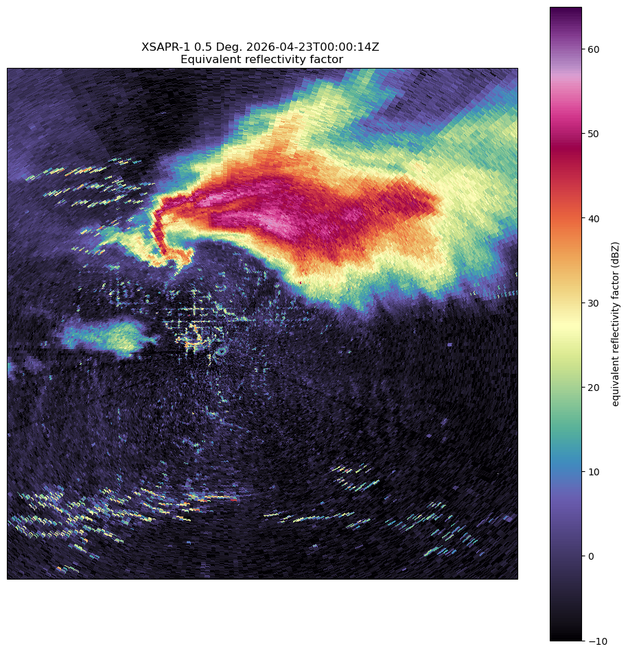

Gridding with Py-ART¶

Gridding is an important workflow to understand when working with radar data! Here, we walk through the steps required.

Antenna vs. Cartesian Coordinates¶

Radar data, by default, is stored in a polar (or antenna) coordinate system, with the data coordinates stored as an angle (ranging from 0 to 360 degrees with 0 == North), and a radius from the radar, and an elevation which is the angle between the ground and the ground.

This format can be challenging to plot, since it is scan/radar specific. Also, it can make comparing with model data, which is on a lat/lon grid, challenging since one would need to transform the model daa cartesian coordinates to polar/antenna coordiantes.

Fortunately, PyART has a variety of gridding routines, which can be used to grid your data to a Cartesian grid. Once it is in this new grid, one can easily slice/dice the dataset, and compare to other data sources.

Why is Gridding Important?¶

Gridding is essential to combining multiple data sources (ex. multiple radars), and comparing to other data sources (ex. model data). There are also decisions that are made during the gridding process that have a large impact on the regridded data - for example:

What resolution should my grid be?
Which interpolation routine should I use?
How smooth should my interpolated data be?

While there is not always a right or wrong answer, it is important to understand the options available, and document which routine you used with your data! Also - experiment with different options and choose the best for your use case!

The Grid Object¶

We can transform our data into this grid object, from the radars, using pyart.map.grid_from_radars().

Beforing gridding our data, we need to make a decision about the desired grid resolution and extent. For example, one might imagine a grid configuration of:

Grid extent/limits
- 20 km in the x-direction (north/south)
- 20 km in the y-direction (west/east)
- 15 km in the z-direction (vertical)
500 m spatial resolution

The pyart.map.grid_from_radars() function takes the grid shape and grid limits as input, with the order (z, y, x).

Let’s setup our configuration, setting our grid extent first, with the distance measured in meters

z_grid_limits = (500.,15_000.)
y_grid_limits = (-30_000.,30_000.)
x_grid_limits = (-30_000.,30_000.)

Now that we have our grid limits, we can set our desired resolution (again, in meters)

grid_resolution = 500

Let’s compute our grid shape - using the extent and resolution to compute the number of grid points in each direction.

def compute_number_of_points(extent, resolution):
    return int((extent[1] - extent[0])/resolution)

Now that we have a helper function to compute this, let’s apply it to our vertical dimension

z_grid_points = compute_number_of_points(z_grid_limits, grid_resolution)
z_grid_points

29

We can apply this to the horizontal (x, y) dimensions as well.

x_grid_points = compute_number_of_points(x_grid_limits, grid_resolution)
y_grid_points = compute_number_of_points(y_grid_limits, grid_resolution)

print(z_grid_points,
      y_grid_points,
      x_grid_points)

29 120 120

Use our configuration to grid the data!¶

Now that we have the grid shape and grid limits, let’s grid up our radar!

grid = pyart.map.grid_from_radars([radar],
                                  grid_shape=(z_grid_points,
                                              y_grid_points,
                                              x_grid_points),
                                  grid_limits=(z_grid_limits,
                                               y_grid_limits,
                                               x_grid_limits),
                                 )
grid

<pyart.core.grid.Grid at 0x17fa3ca10>

Plot the Grid Object¶

Plot a horizontal view of the data¶

We can use the GridMapDisplay from pyart.graph to visualize our regridded data, starting with a horizontal view (slice along a single vertical level)

display = pyart.graph.GridMapDisplay(grid)
display.plot_grid('reflectivity',
                  level=0,
                  vmin=-20,
                  vmax=60,
                  cmap='ChaseSpectral')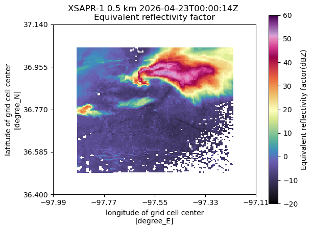

Plot a Latitudinal Slice¶

We can also slice through a single latitude or longitude!

display.plot_latitude_slice('reflectivity',
                            lat=36.955,
                            vmin=-20,
                            vmax=60,
                            cmap='ChaseSpectral')
plt.xlim([-20, 20]);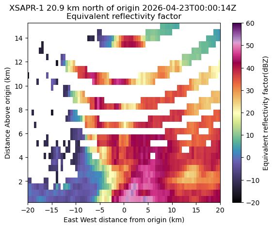

Plot with Xarray¶

Another neat feature of the Grid object is that we can transform it to an xarray.Dataset!

ds = grid.to_xarray()
ds

Now, our plotting routine is a one-liner, starting with the horizontal slice:

ds.isel(z=0).reflectivity.plot(cmap='ChaseSpectral',
                               vmin=-20,
                               vmax=60);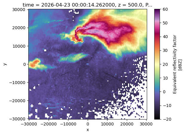

And a vertical slice at a given y dimension (latitude)

ds.sel(y=19000,
       method='nearest').reflectivity.plot(cmap='ChaseSpectral',
                                           vmin=-20,
                                           vmax=60);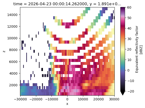

What’s Next¶

In the next few notebooks, we walk through applying data cleaning methods, and advanced visualization methods!

References¶

Helmus, J. J., & Collis, S. M. (2016). The Python ARM Radar Toolkit (Py-ART), a Library for Working with Weather Radar Data in the Python Programming Language. Journal of Open Research Software, 4(1), e25. 10.5334/jors.119
Grover, M., Mühlbauer, K., Goudenhoofdt, E., Syed, H. A., Ladino, A., Jackson, R., & Wolfensberger, D. (2026). openradar/xradar: xradar v0.12.0 (0.12.0) [Computer software]. 10.5281/zenodo.7091737
Sherman, Z., Grover, M., Jackson, R., Collis, S., O’Brien, J., Homeyer, C. R., Chase, R. J., Lang, T. J., Stechman, D. M., Sockol, A., Muehlbauer, K., Thielen, J., Theisen, A., Gardner, S., & Michelson, D. (2024). Effective Visualization of Radar Data for Users Impacted by Color Vision Deficiency. Bulletin of the American Meteorological Society, 105(8). 10.1175/BAMS-D-23-0056.1
Bharadwaj, N., Hardin, J., Isom, B., Johnson, K., Lindenmaier, I., Matthews, A., Nelson, D., Feng, Y.-C., Wendler, T., Rocque, M., & et al. (2026). X-Band Scanning ARM Precipitation Radar (XSAPRCFR), 2026-04-23 to 2026-04-24, Southern Great Plains (SGP), Deer Creek, OK (Intermediate) (I6). In Atmospheric Radiation Measurement (ARM) user facility. 10.5439/1463663

Py-ART Basics with Xradar

Py-ART Basics with Xradar¶

Overview¶

History of the Python ARM Radar Toolkit (Py-ART)¶

What can Py-ART Do?¶

Py-ART 2.0¶

Prerequisites¶

Imports¶

Reading in Data Using Py-ART and xradar¶

Reading data in using xradar.io.open_¶

Investigate the xradar object¶

Extract a sample data field¶

Plotting our Radar Data¶

An Overview of Py-ART Plotting Utilities¶

Use the RadarMapDisplay with our data¶

Gridding with Py-ART¶

Antenna vs. Cartesian Coordinates¶

Why is Gridding Important?¶

The Grid Object¶

Use our configuration to grid the data!¶

Plot the Grid Object¶

Plot a horizontal view of the data¶

Plot a Latitudinal Slice¶

Plot with Xarray¶

What’s Next¶

Reading data in using `xradar.io.open_`¶

Investigate the `xradar` object¶