
ACT Basics

Overview
The Atmospheric data Community Toolkit (ACT) is an open source Python toolkit for working with atmospheric time-series datasets of varying dimensions (Theisen et al. (2026)). The toolkit is meant to have functions for every part of the scientific process:
discovery,
IO,
quality control,
corrections,
retrievals,
visualization,
and analysis.
It is meant to be a community platform for sharing code with the goal of reducing duplication of effort and better connecting the science community with programs such as the Atmospheric Radiation Measurement (ARM) User Facility.
This tutorial will provide an introduction to ACT using the ARM Surface Meteorological Instrumentation MET at the Southern Great Plains (SGP) to investigate temperature trends over the data record.
Intro to ACT
Instrument Overview
Downloading and Reading in Data
Quality Controlling Data
Visualizing Data
Monthly Temperature Trend Analysis
Prerequisites
This notebook will rely heavily on Python and the Atmospheric data Community Toolkit (ACT). Don’t worry if you don’t have experience with either, this notebook will walk you though what you need to know.
| Concepts | Importance | Notes |
|---|---|---|
| ACT | Helpful | |
| Xarray Basics | Helpful | Multi-dimensional arrays |
| Matplotlib Basics | Helpful | Basic plotting |
| NumPy Basics | Helpful | Basic arrays |
Time to learn: 15 Minutes
System requirements:
Python 3.11 or latest
ACT v2.0.0 or latest
numpy
xarray
matplotlib
Intro to ACT
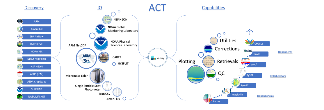
The Atmospheric data Community Toolkit (ACT) is an open-source Python toolkit for exploring and analyzing atmospheric time-series datasets. Examples can be found in the ACT Example Gallery. The toolkit has modules for many different parts of the scientific process, including:
Enhanced Skew-T plot from ARM’s Southern Great Plains Site (SGP)
Data Discovery (act.discovery)¶The discovery module houses functions to download or access data from different groups. Currently it includes function to get data for ARM, NOAA, EPA, NEON, and more! Input/Output (act.io)¶io contains functions for reading and writing data from various sources and formats. Visualization (act.plotting)¶plotting contains various routines, built on matplotlib, to help visualize and explore data. These include
Corrections (act.corrections)¶corrections apply different corrections to data based on need. A majority of the existing corrections are for lidar data. Quality Control (act.qc)¶The qc module has a lot of functions for working with quality control information, apply new tests, or filtering data based on existing tests. We will explore some of that functionality in this notebook. Retrievals (act.retrievals)¶There are many cases in which some additional calculations are necessary to get more value from the instrument data. The retrievals module houses some functions for performing these advanced calculations. Utilities (act.utils)¶The utils module has a lot of general utilities to help with the data. Some of these include adding in a solar variable to indicate day/night (useful in filtering data), unit conversions, decoding WMO weather codes, performing weighted averaging, etc... | 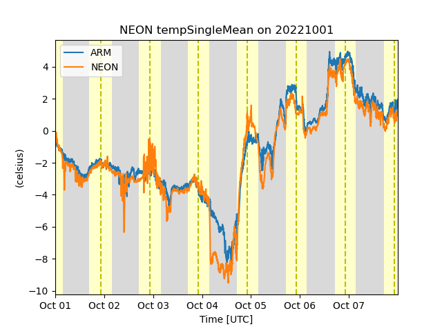 ARM and NEON data from Utquivaik, AK 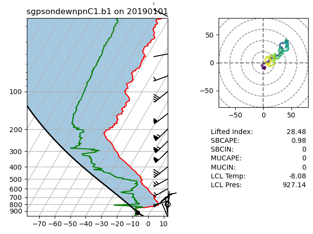 |
Instrument Overview
Surface Meteorological Instrumentation (MET) - Kyrouac et al. (2026)
The ARM Surface Meteorology Systems (MET) use mainly conventional in situ sensors to obtain 1-minute statistics of surface wind speed, wind direction, air temperature, relative humidity, barometric pressure, and rain-rate. Learn more
Imports
Let’s get started with some data! But first, we need to import some libraries.
# Uncomment if running on CoLab
##!pip install act-atmos>=2.2.23
import os
import numpy as np
import xarray as xr
import matplotlib.pyplot as plt
import matplotlib.colors as colors
import getpass
import act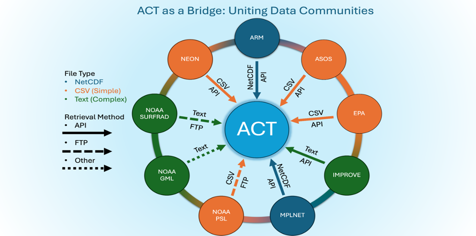
Downloading and Reading ARM’s NetCDF Data
ARM’s standard file format is NetCDF (network Common Data Form) which makes it very easy to work with in Python! ARM data are available through a data portal called Data Discovery or through a webservice. If you didn’t get your username and token earlier, please go back and see the Prerequisites!
Let’s download some of the MET data first from two facilities[1]!
# Note - recommended ARM Live token to be set as an environmental variable

# Check for env variables, otherwise set your username and token here!
if "ARM_USERNAME" in os.environ:
    arm_username = os.getenv("ARM_USERNAME")
else:
    arm_username = input("Enter ARM username: ").strip()
if "ARM_TOKEN" in os.environ:
    arm_token = os.getenv("ARM_TOKEN")
else:
    arm_token = getpass.getpass("Enter ARM token (hidden): ").strip()

# Set the datastream and start/enddates
cf_datastream = 'sgpmetE13.b1'
ef_datastream = "sgpmetE39.b1"

startdate = '2026-04-01'
enddate = '2026-04-30'

# Use ACT to easily download the data.  Watch for the data citation!  Show some support
# for ARM's instrument experts and cite their data if you use it in a publication
result_cf_met = act.discovery.download_arm_data(arm_username, arm_token, cf_datastream, startdate, enddate)
result_ef_met = act.discovery.download_arm_data(arm_username, arm_token, ef_datastream, startdate, enddate)
[DOWNLOADING] sgpmetE13.b1.20260401.000000.cdf
[DOWNLOADING] sgpmetE13.b1.20260402.000000.cdf
[DOWNLOADING] sgpmetE13.b1.20260403.000000.cdf
[DOWNLOADING] sgpmetE13.b1.20260404.000000.cdf
[DOWNLOADING] sgpmetE13.b1.20260405.000000.cdf
[DOWNLOADING] sgpmetE13.b1.20260406.000000.cdf
[DOWNLOADING] sgpmetE13.b1.20260407.000000.cdf
[DOWNLOADING] sgpmetE13.b1.20260408.000000.cdf
[DOWNLOADING] sgpmetE13.b1.20260409.000000.cdf
[DOWNLOADING] sgpmetE13.b1.20260410.000000.cdf
[DOWNLOADING] sgpmetE13.b1.20260411.000000.cdf
[DOWNLOADING] sgpmetE13.b1.20260412.000000.cdf
[DOWNLOADING] sgpmetE13.b1.20260413.000000.cdf
[DOWNLOADING] sgpmetE13.b1.20260414.000000.cdf
[DOWNLOADING] sgpmetE13.b1.20260415.000000.cdf
[DOWNLOADING] sgpmetE13.b1.20260415.130000.cdf
[DOWNLOADING] sgpmetE13.b1.20260415.152300.cdf
[DOWNLOADING] sgpmetE13.b1.20260415.160000.cdf
[DOWNLOADING] sgpmetE13.b1.20260416.000000.cdf
[DOWNLOADING] sgpmetE13.b1.20260417.000000.cdf
[DOWNLOADING] sgpmetE13.b1.20260418.000000.cdf
[DOWNLOADING] sgpmetE13.b1.20260419.000000.cdf
[DOWNLOADING] sgpmetE13.b1.20260420.000000.cdf
[DOWNLOADING] sgpmetE13.b1.20260421.000000.cdf
[DOWNLOADING] sgpmetE13.b1.20260422.000000.cdf
[DOWNLOADING] sgpmetE13.b1.20260423.000000.cdf
[DOWNLOADING] sgpmetE13.b1.20260424.000000.cdf
[DOWNLOADING] sgpmetE13.b1.20260425.000000.cdf
[DOWNLOADING] sgpmetE13.b1.20260426.000000.cdf
[DOWNLOADING] sgpmetE13.b1.20260427.000000.cdf
[DOWNLOADING] sgpmetE13.b1.20260428.000000.cdf
[DOWNLOADING] sgpmetE13.b1.20260429.000000.cdf
[DOWNLOADING] sgpmetE13.b1.20260430.000000.cdf
If you use these data to prepare a publication, please cite:
Kyrouac, J., Shi, Y., & Tuftedal, M. Surface Meteorological Instrumentation
(MET), 2026-04-01 to 2026-04-30, Southern Great Plains (SGP), Lamont, OK
(Extended and Co-located with C1) (E13). Atmospheric Radiation Measurement (ARM)
User Facility. https://doi.org/10.5439/1786358
[DOWNLOADING] sgpmetE39.b1.20260401.000000.cdf
[DOWNLOADING] sgpmetE39.b1.20260402.000000.cdf
[DOWNLOADING] sgpmetE39.b1.20260403.000000.cdf
[DOWNLOADING] sgpmetE39.b1.20260404.000000.cdf
[DOWNLOADING] sgpmetE39.b1.20260405.000000.cdf
[DOWNLOADING] sgpmetE39.b1.20260406.000000.cdf
[DOWNLOADING] sgpmetE39.b1.20260407.000000.cdf
[DOWNLOADING] sgpmetE39.b1.20260408.000000.cdf
[DOWNLOADING] sgpmetE39.b1.20260409.000000.cdf
[DOWNLOADING] sgpmetE39.b1.20260410.000000.cdf
[DOWNLOADING] sgpmetE39.b1.20260411.000000.cdf
[DOWNLOADING] sgpmetE39.b1.20260412.000000.cdf
[DOWNLOADING] sgpmetE39.b1.20260413.000000.cdf
[DOWNLOADING] sgpmetE39.b1.20260414.000000.cdf
[DOWNLOADING] sgpmetE39.b1.20260415.000000.cdf
[DOWNLOADING] sgpmetE39.b1.20260416.000000.cdf
[DOWNLOADING] sgpmetE39.b1.20260417.000000.cdf
[DOWNLOADING] sgpmetE39.b1.20260418.000000.cdf
[DOWNLOADING] sgpmetE39.b1.20260419.000000.cdf
[DOWNLOADING] sgpmetE39.b1.20260420.000000.cdf
[DOWNLOADING] sgpmetE39.b1.20260421.000000.cdf
[DOWNLOADING] sgpmetE39.b1.20260422.000000.cdf
[DOWNLOADING] sgpmetE39.b1.20260423.000000.cdf
[DOWNLOADING] sgpmetE39.b1.20260424.000000.cdf
[DOWNLOADING] sgpmetE39.b1.20260425.000000.cdf
[DOWNLOADING] sgpmetE39.b1.20260426.000000.cdf
[DOWNLOADING] sgpmetE39.b1.20260427.000000.cdf
[DOWNLOADING] sgpmetE39.b1.20260428.000000.cdf
[DOWNLOADING] sgpmetE39.b1.20260429.000000.cdf
[DOWNLOADING] sgpmetE39.b1.20260430.000000.cdf
If you use these data to prepare a publication, please cite:
Kyrouac, J., Shi, Y., & Tuftedal, M. Surface Meteorological Instrumentation
(MET), 2026-04-01 to 2026-04-30, Southern Great Plains (SGP), Morrison, OK
(Extended) (E39). Atmospheric Radiation Measurement (ARM) User Facility.
https://doi.org/10.5439/1786358
# Let's read in the data using ACT and check out the data
ds_cf_met = act.io.read_arm_netcdf(result_cf_met)
ds_ef_met = act.io.read_arm_netcdf(result_ef_met)

ds_cf_met# Since ACT is built upon xarray, we can use xarray's built in plotting to quickly visualize the data
ds_cf_met['temp_mean'].plot()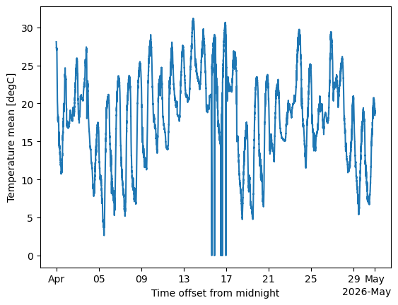
# We can also use xarray's built in slicing to quickly subset the data.
# Let's look at some suspect data points in the temperature data
ds_cf_met['temp_mean'].sel(time=slice('2026-04-15T00:00', '2026-04-17T00:00')).plot()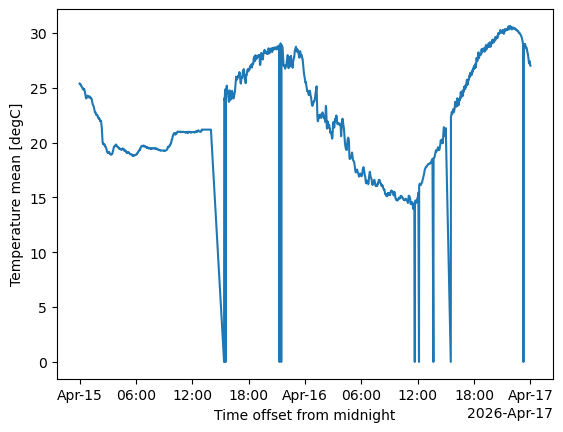
Quality Controlling Data
ARM has multiple methods that it uses to communicate data quality information out to the users. One of these methods is through “embedded QC” variables. These are variables within the file that have information on automated tests that have been applied. Many times, they include Min, Max, and Delta tests but as is the case with the Aerosol Observing System (AOS) instruments, there can be more complicated tests that are applied.
The results from all these different tests are stored in a single variable using bit-packed QC. We won’t get into the full details here, but it’s a way to communicate the results of multiple tests in a single integer value by utilizing binary and bits! You can learn more about bit-packed QC here but ACT also has many of the tools for working with ARM QC.
Other Sources of Quality Control
ARM also communicates problems with the data quality through Data Quality Reports (DQR). These reports are normally submitted by the instrument mentor when there’s been a problem with the instrument. The categories include:
Data Quality Report Categories
Missing: Data are not available or set to -9999
Suspect: The data are not fully incorrect but there are problems that increases the uncertainty of the values. Data should be used with caution.
Bad: The data are incorrect and should not be used.
Note: Data notes are a way to communicate information that would be useful to the end user but does not rise to the level of suspect or bad data
Additionally, data quality information can be found in the Instrument Handbooks, which are included on most instrument pages. Here is an example of the MET handbook.
# We can see that there's some missing data in the plot above so let's take a look at the embedded QC!
# First, for many of the ACT QC features, we need to get the dataset more to CF standard and that
# involves cleaning up some of the attributes and ways that ARM has historically handled QC
ds_cf_met.clean.cleanup()

# Query the ARM DQR Webservice
variable = 'temp_mean'
ds_cf_met = act.qc.add_dqr_to_qc(ds_cf_met, variable=variable)ds_cf_met# Next, let's take a look at visualizing the quality control information
# Create a plotting display object with 2 plots
display = act.plotting.TimeSeriesDisplay(ds_cf_met, figsize=(15, 10), subplot_shape=(2,))
# Plot up the variable in the first plot
display.plot(variable, subplot_index=(0,))
# Plot up a day/night background
display.day_night_background(subplot_index=(0,))
# Plot up the QC variable in the second plot
display.qc_flag_block_plot(variable, subplot_index=(1,))
plt.show()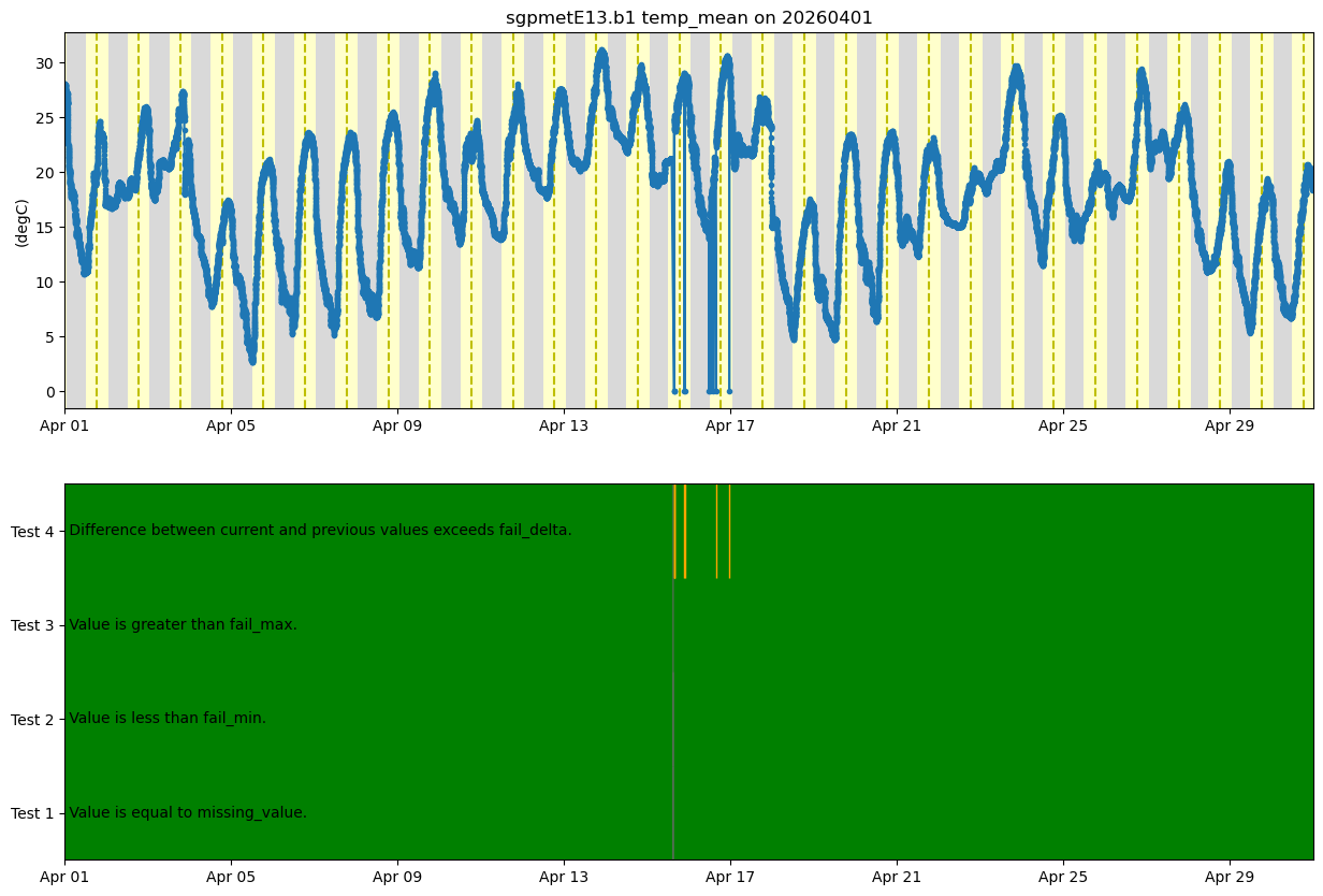
# Next, let's take a look at visualizing the quality control information
# Create a plotting display object with 2 plots
display = act.plotting.TimeSeriesDisplay(ds_cf_met.sel(time=slice('2026-04-15T00:00', '2026-04-17T00:00')), figsize=(15, 10), subplot_shape=(2,))

# Plot up the variable in the first plot
display.plot(variable, subplot_index=(0,))

# Plot up a day/night background
display.day_night_background(subplot_index=(0,))

# Plot up the QC variable in the second plot
display.qc_flag_block_plot(variable, subplot_index=(1,))
plt.show()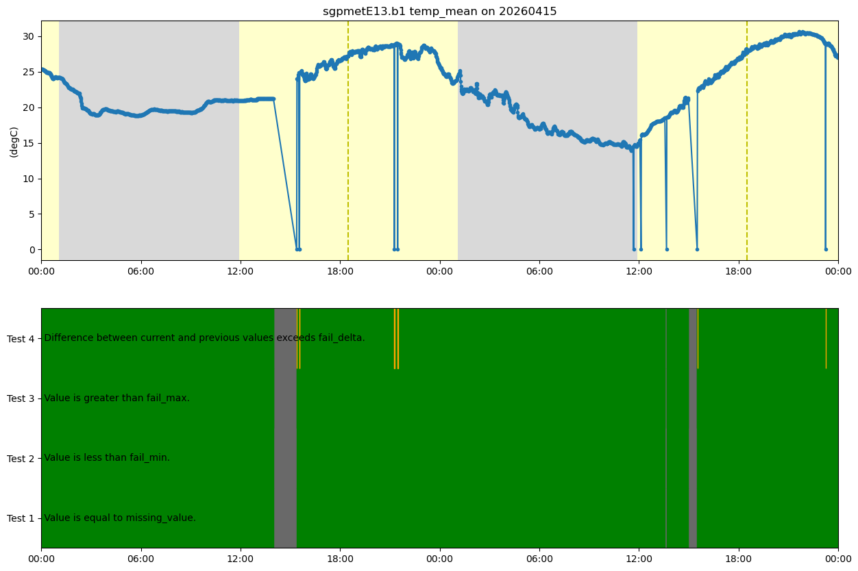
Visualizing Data
We’ve already worked with visualizing the data in basic ways but what other options are there in ACT? This section will show you how to create a variety of different plots. More plotting examples can be found in ACT’s Documentation.
Multi-Panel Plot
This example shows how to plot multiple datastreams together (both METS) on a multi-panel plot.
#And plot again!
# Create a plotting display object with 2 plots
# Note we have to create a dictionary of datasets to pass in
display = act.plotting.TimeSeriesDisplay({'CF': ds_cf_met, 'EF': ds_ef_met}, figsize=(15, 10), subplot_shape=(2,))

# Plot up the variable in the first plot
# Need to specify the dsname so it knows which dataset
# to use for this data.  This is helpful when datasets
# have similar variable names
display.plot('temp_mean', dsname='CF', subplot_index=(0,))
ax1 = display.axes[0].twinx()
ax1.plot(ds_cf_met.time, ds_cf_met.tbrg_precip_total, color='orange')

# Plot up the EF-MET temperature and precipitation
display.plot('temp_mean', dsname='EF', subplot_index=(1,))
ax2 = display.axes[1].twinx()
ax2.plot(ds_ef_met.time, ds_ef_met.tbrg_precip_total, color='orange')

# Plot up a day/night background
display.day_night_background(dsname='CF', subplot_index=(0,))
display.day_night_background(dsname='EF', subplot_index=(1,))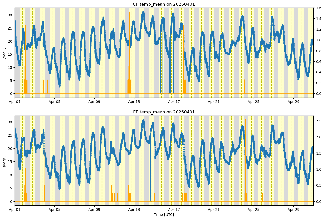
Adding some customization
Let’s make this plot a little nicer and easier to read. We can use a mix of ACT and Matplotlib to help
#And plot again!
# Create a plotting display object with 2 plots
# Note we have to create a dictionary of datasets to pass in
display = act.plotting.TimeSeriesDisplay({'CF': ds_cf_met, 'EF': ds_ef_met}, figsize=(15, 10), subplot_shape=(2,))

# Let's accumulate the precipitation using ACT to make this easier to read
ds_cf_met = act.utils.data_utils.accumulate_precip(ds_cf_met, 'tbrg_precip_total')
ds_ef_met = act.utils.data_utils.accumulate_precip(ds_ef_met, 'tbrg_precip_total')

# Let's add in titles and more to the SMPS plot
title = 'MET Temperature and Precipitation at SGP CF (EF13)'
display.plot('temp_mean', dsname='CF', subplot_index=(0,), set_title=title,
             ylabel='Temperature (C)', color='black')
display.set_yrng([0, 35], subplot_index=(0,))
ax1 = display.axes[0].twinx()
ax1.plot(ds_cf_met.time, ds_cf_met.tbrg_precip_total_accumulated, color='red')
ax1.set_ylabel('Precipitation (mm)')
ax1.set_ylim([0, 140.0])

# Plot up the MET btemperature and precipitation
title = 'MET Temperature and Cumulative Precipitation at SGP EF39'
display.plot('temp_mean', dsname='EF', subplot_index=(1,), set_title=title, color='black')
display.set_yrng([0, 35], subplot_index=(1,))
ax2 = display.axes[1].twinx()
ax2.plot(ds_ef_met.time, ds_ef_met.tbrg_precip_total_accumulated, color='red')
ax2.set_ylabel('Precipitation (mm)')
ax2.set_ylim([0, 140.0])

# Plot up a day/night background
display.day_night_background(dsname='CF', subplot_index=(0,))
display.day_night_background(dsname='EF', subplot_index=(1,))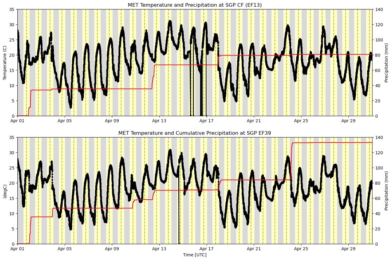
Distribution Display
For the example, we will go over some functions within ACT’s distribution display. Functions such as, the stacked bar plot, scatter and groupby.
# First, let's plot up a histogram of the data
# All the ACT plotting is very similar to what we
# did earlier, first we create a display object
display = act.plotting.DistributionDisplay(ds_cf_met)

# And then we can plot the data!  Note that we are passing a range into the
# histogram function to set the min/max range of the data
display.plot_stacked_bar('temp_mean', hist_kwargs={'range': [4, 20]})
plt.show()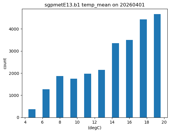
# Let's directly compare the two datasets using a scatter plot.
# First we need to clean up the datasets and average to the same time grid
# Once again, we take advantage of the xarray data structures and use xarray's resample function
ds_cf_qc = ds_cf_met.where(ds_cf_met.temp_mean > 0).resample(time='10min').nearest()
ds_ef_qc = ds_ef_met.where(ds_ef_met.temp_mean > 0).resample(time='10min').nearest()

# Note - plenty of ways to do this, but adding a suffix to distinguish between two sites
suffix = "_ef"
exclude = ["base_time", "time_bounds", "time_offset", "lat", "lon", "alt"]
ds_ef_qc = ds_ef_qc.rename_vars({
    var: f"{var}{suffix}"
    for var in ds_ef_qc.data_vars
    if var not in exclude
})

# quick check to make sure we've eliminated the questionable data
ds_cf_qc.temp_mean.plot(label='CF-MET')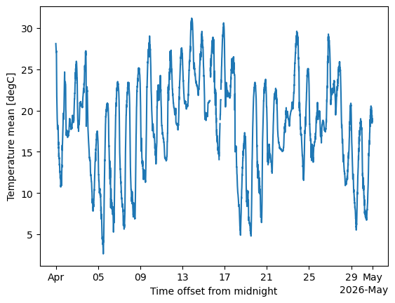
# Combine the datasets together using xarray's merge function.
ds_combined = xr.merge([ds_cf_qc, ds_ef_qc], compat='override')

# Next up, let's do some scatter plots to compare some variables
# Scatter plots are also found in the DistributionDisplay module
display = act.plotting.DistributionDisplay(ds_combined)
display.set_xrng([0, 40])
display.set_yrng([0, 40])

# And then we can plot the data!
display.plot_scatter('temp_mean',
                     'temp_mean_ef',
                     m_field='wdir_vec_mean',
                     marker='x',
                     cbar_label=r'Wind Direction ($^\circ$)',
)

# Display the 1:1 ratio line
display.set_ratio_line()

plt.show()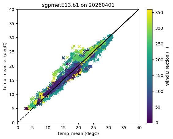
Data Rose Plots
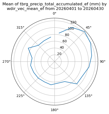
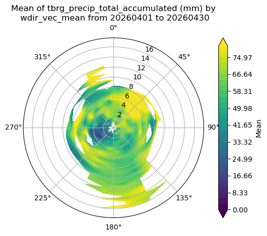
If your data may be wind speed or direction dependent, these plots can help inform where the influences may be coming from (or confirm there are no blocking QC issues). For this example, let’s see if tipping bucket rain guage data are dependent on wind direction
# Plot out the data rose using the WindRose display object
display = act.plotting.WindRoseDisplay(ds_combined)
display.plot_data('wdir_vec_mean_ef', 'wspd_vec_mean_ef', 'tbrg_precip_total_accumulated_ef', num_dirs=20, plot_type='line', line_plot_calc='mean')
plt.show()
/Users/jrobrien/.vscode-micromamba/envs/arm-summer-school-2026-dev/lib/python3.11/site-packages/act/plotting/windrosedisplay.py:358: RuntimeWarning: Mean of empty slice
arr.append(np.nanmean(data[idx]))
# Plot out the data rose using the WindRose display object
display = act.plotting.WindRoseDisplay(ds_combined)

# Let's try a different type of data rose type that is using contours amd the polar y axis is wind speed
# depending on wind direction and speed
display.plot_data('wdir_vec_mean', 'wspd_vec_mean', 'tbrg_precip_total_accumulated', num_dirs=20, plot_type='contour', contour_type='mean')
plt.show()
/Users/jrobrien/.vscode-micromamba/envs/arm-summer-school-2026-dev/lib/python3.11/site-packages/act/plotting/windrosedisplay.py:429: RuntimeWarning: Mean of empty slice
mean_data[i, j] = np.nanmean(data[idx])
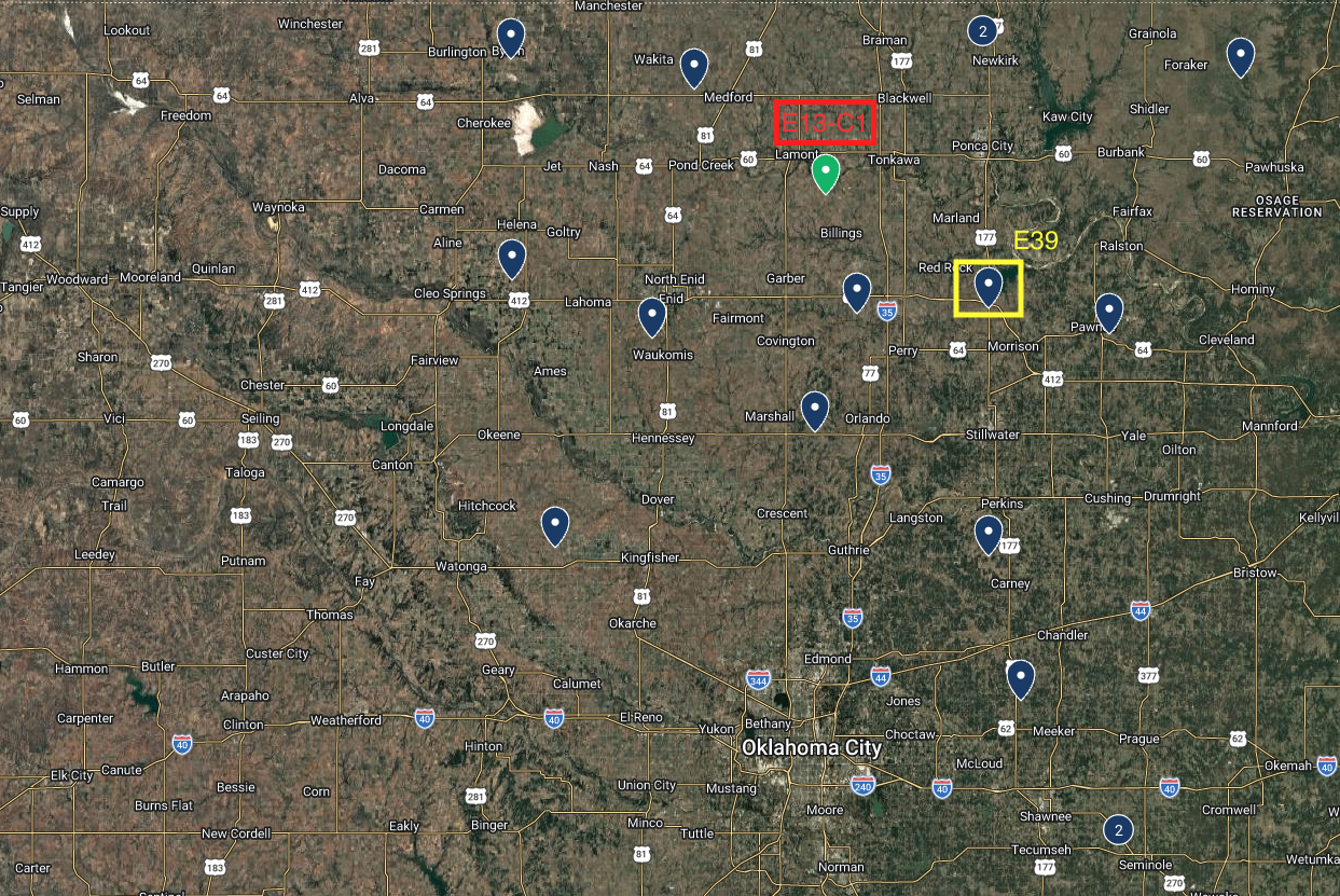
Location of MET Measurements at SGP’s central and extended facilities
- Theisen, A., Kehoe, K., Sherman, Z., Jackson, B., Grover, M., Sockol, A. J., Godine, C., Hemedinger, J., O’Brien, J., Kyrouac, J., Silber, I., Levin, M., Shah, C. H., Gibson, L. D., & dennyh ssec. (2026). ARM-DOE/ACT: ACT Release Version 2.3.0 (v2.3.0) [Computer software]. Zenodo. 10.5281/zenodo.18356119
- Kyrouac, J., Shi, Y., & Tuftedal, M. (2026). Surface Meteorological Instrumentation (MET), 1993-07-21 to 2026-04-30, Southern Great Plains (SGP), Lamont, OK (Extended and Co-located with C1) (E13). In Atmospheric Radiation Measurement (ARM) user facility. 10.5439/1786358