Py-ART Corrections¶

Overview¶

We have previously covered reading of X-Band ARM Scanning Preciptiation Radar (XSAPR) (Bharadwaj et al. (2026)) data and displaying convective cells associated with the 23 April 2026 Enid, Oklahoma Enhanced Fujita (EF) Scale (EF-4) tornado outbreak.

Within this notebook, we will cover the pyart.correct module for correcting radar moments while in antenna coordinates. Specifically, this notebook will cover:

Intro to radar aliasing.
Calculation of velocity texture using Py-ART
Dealiasing the velocity field within the 23 April 2026 Enid supercells.

Prerequisites¶

Concepts	Importance	Notes
Py-ART Basics	Helpful	Basic features
Weather Radar Basics	Helpful	Background Information
Matplotlib Basics	Helpful	Basic plotting
NumPy Basics	Helpful	Basic arrays
Xarray Basics	Helpful	Multi-dimensional arrays

Time to learn: 15 minutes

An Overview of Aliasing¶

The radial velocity measured by the radar is mesasured by detecting the phase shift between the transmitted pulse and the pulse recieved by the radar. However, using this methodology, it is only possible to detect phase shifts within ±2π due to the periodicity of the transmitted wave.

Therefore, for example, a phase shift of 3π would erroneously be detected as a phase shift of −π and give an incorrect value of velocity when retrieved by the radar. This phenomena is called aliasing. The maximium unambious velocity that can be detected by the radar before aliasing occurs is called the Nyquist velocity.

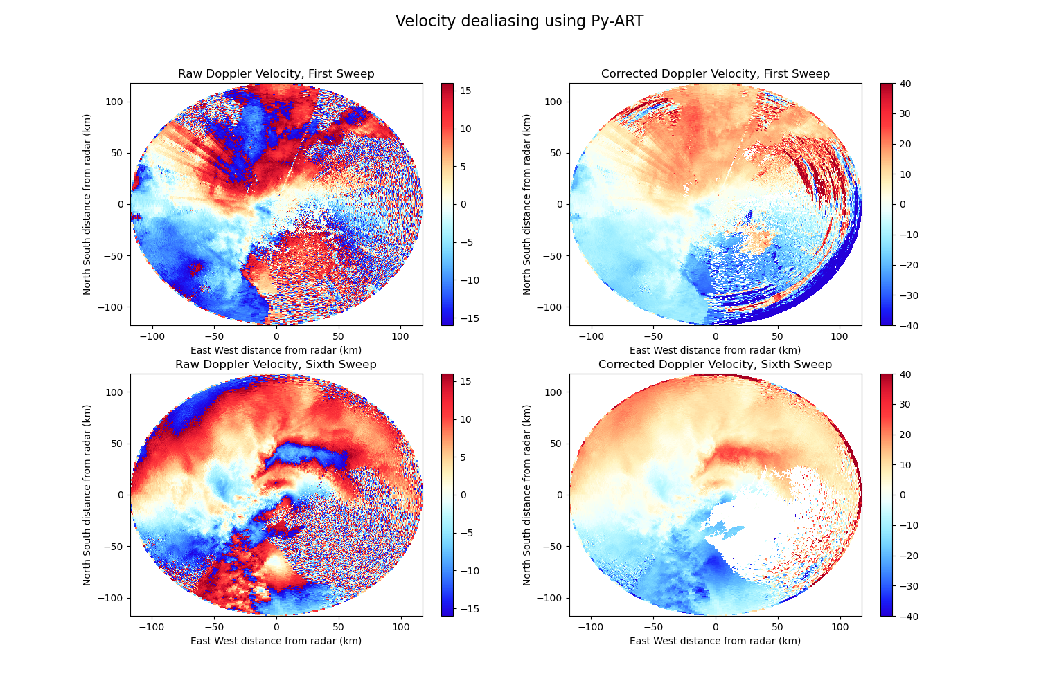
In the above example, you will see an example of aliasing occurring, where the values of +15 m/s abruptly transition into a region of -15 m/s, with -5 m/s in the middle of the region around 50-100km North of the radar.

# Uncomment if running on CoLab
##!pip install arm_pyart>=2.2.0
##!pip install xradar>=0.12.0

# Uncomment if running on CoLab
##import pathlib
##from pathlib import Path
##import gdown

##DATA_LINK = "1QLRRZMJ-HRQpbhATPqLfF8byJmnYWXzv"
##CREATE_BASE = pathlib.Path("../data")
##CREATE_BASE.mkdir(parents=True, exist_ok=True)
##gdown.download(id=DATA_LINK, output=str(CREATE_BASE / "sgpxsaprcfrI6.a1.20260423.233233.nc"), quiet=False)

Calculating Velocity Texture with Py-ART¶

import os
import warnings

import cartopy.crs as ccrs
import matplotlib.pyplot as plt
import numpy as np
import xarray as xr

import pyart
from pyart.testing import get_test_data
import xradar as xd

warnings.filterwarnings('ignore')


## You are using the Python ARM Radar Toolkit (Py-ART), an open source
## library for working with weather radar data. Py-ART is partly
## supported by the U.S. Department of Energy as part of the Atmospheric
## Radiation Measurement (ARM) Climate Research Facility, an Office of
## Science user facility.
##
## If you use this software to prepare a publication, please cite:
##
##     JJ Helmus and SM Collis, JORS 2016, doi: 10.5334/jors.119

Read in the Data¶

# As in the Py-ART Basics notebook, we begin by loading a XSAPR CF-Radial file for our period of interest. 
# Adjust the base path and file name as needed to point to the location of the data on your system (or Colab)
base_path = "../data/"
file = "sgpxsaprcfrI6.a1.20260423.233233.nc"
dt = xd.io.open_cfradial1_datatree(base_path + file)
radar = pyart.xradar.Xradar(dt)

radar

Plot a quick-look of reflectivity and velocity¶

We can start by taking a quick look at the reflectivity and velocity fields. Notice how the velocity field is rather messy, indicated by the speckles and high/low values directly next to each other

fig = plt.figure(figsize=[8, 10])
ax = plt.subplot(211, projection=ccrs.PlateCarree())
display = pyart.graph.RadarMapDisplay(radar)
display.plot_ppi_map('reflectivity',
                     ax=ax,
                     sweep=1,
                     resolution='50m',
                     vmin=0,
                     vmax=60, 
                     projection=ccrs.PlateCarree(),    
                     cmap="ChaseSpectral",
                     min_lat=36.3,
                     max_lat=36.9,
                     min_lon=-97.8,
                     max_lon=-97.20)

ax2 = plt.subplot(2,1,2,projection=ccrs.PlateCarree())
display = pyart.graph.RadarMapDisplay(radar)
display.plot_ppi_map('mean_doppler_velocity',
                     ax=ax2,
                     sweep=1,
                     resolution='50m',
                     vmin=-12,
                     vmax=12, 
                     projection=ccrs.PlateCarree(),
                     cmap='balance',
                     min_lat=36.3,
                     max_lat=36.9,
                     min_lon=-97.8,
                     max_lon=-97.20)
plt.show()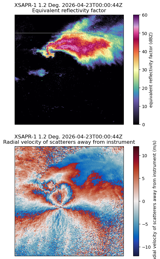

Calculate Velocity Texture¶

First, for dealiasing to work efficiently, we need to use a GateFilter.

Notice that, this time, the data shown does not give us a nice gate_id. This is what raw data looks like, and we need to do some preprocessing on the data to remove noise and clutter.

Thankfully, Py-ART gives us the capability to do this.

As a simple filter in this example, we will first calculate the velocity texture using Py-ART’s calculate_velocity_texture function. The velocity texture is the standard deviation of velocity surrounding a gate. This will be higher in the presence of noise.

Let’s investigate this function first...

pyart.retrieve.calculate_velocity_texture?

Signature:
pyart.retrieve.calculate_velocity_texture(
    radar,
    vel_field=None,
    wind_size=3,
    nyq=None,
    check_nyq_uniform=True,
)
Docstring:
Derive the texture of the velocity field.

Parameters
----------
radar: Radar
    Radar object from which velocity texture field will be made.
vel_field : str, optional
    Name of the velocity field. A value of None will force Py-ART to
    automatically determine the name of the velocity field.
wind_size : int or 2-element tuple, optional
    The size of the window to calculate texture from.
    If an integer, the window is defined to be a square of size wind_size
    by wind_size. If tuple, defines the m x n dimensions of the filter
    window.
nyq : float, optional
    The nyquist velocity of the radar. A value of None will force Py-ART
    to try and determine this automatically.
check_nyquist_uniform : bool, optional
    True to check if the Nyquist velocities are uniform for all rays
    within a sweep, False will skip this check. This parameter is ignored
    when the nyq parameter is not None.

Returns
-------
vel_dict: dict
    A dictionary containing the field entries for the radial velocity
    texture.
File:      ~/.vscode-micromamba/envs/arm-summer-school-2026-dev/lib/python3.11/site-packages/pyart/retrieve/simple_moment_calculations.py
Type:      function

Determining the Right Parameters¶

You’ll notice that we need:

Our radar object
The name of our velocity field
The number of gates within our window to use to calculate the texture
The nyquist velocity

We can retrieve the nyquest velocity from our instrument parameters fortunately - using the following syntax!

Calculate Velocity Texture and Filter our Data¶

Now that we have an ide?a of which parameters to pass in, let’s calculate velocity texture!

vel_texture = pyart.retrieve.calculate_velocity_texture(radar,
                                                        vel_field='mean_doppler_velocity',
                                                        nyq=8.525)
vel_texture

{'units': 'meters_per_second',
 'standard_name': 'texture_of_radial_velocity_of_scatters_away_from_instrument',
 'long_name': 'Doppler velocity texture',
 'coordinates': 'elevation azimuth range',
 'data': array([[4.14583856, 4.20702349, 4.20702349, ..., 3.97871742, 3.89128569,
         3.69138473],
        [4.14583856, 4.20702349, 4.24720521, ..., 3.97871742, 3.89128569,
         3.50924729],
        [4.97902753, 4.97902753, 5.13052479, ..., 3.8902026 , 3.8902026 ,
         3.50924729],
        ...,
        [2.21806465, 3.24565856, 4.04686669, ...,        nan,        nan,
                nan],
        [3.03031847, 4.85188931, 4.53731102, ...,        nan,        nan,
                nan],
        [4.85188931, 5.06432979, 5.06432979, ...,        nan,        nan,
                nan]], shape=(6480, 1001))}

# Mask out NaN values for histogram plotting - replacing with high frequency value that will be scaled out
vel_update = np.where(np.isnan(vel_texture['data']), 20, vel_texture['data'])
vel_texture['data'] = vel_update

The pyart.retrieve.calculate_velocity_texture function results in a data dictionary, including the actual data, as well as metadata. We can add this to our radar object, by using the radar.add_field method, passing the name of our new field ("texture"), the data dictionary (vel_texture), and a clarification that we want to replace the existing velocity texture field if it already exists in our radar object (replace_existing=True)

radar.add_field('texture', vel_texture, replace_existing=True)

Plot our Velocity Texture Field¶

Now that we have our velocity texture field added to our radar object, let’s plot it!

fig = plt.figure(figsize=[8, 8])
display = pyart.graph.RadarMapDisplay(radar)
display.plot_ppi_map('texture',
                     sweep=1,
                     resolution='50m',
                     vmin=0,
                     vmax=10, 
                     projection=ccrs.PlateCarree(),
                     cmap='balance')
plt.show()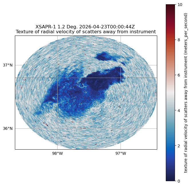

Determine a Suitable Velocity Texture Threshold¶

Plot a histogram of velocity texture to get a better idea of what values correspond to hydrometeors and what values of texture correspond to artifacts.

In the below example, a threshold of 2.5 would eliminate most of the peak corresponding to noise around 6 while preserving most of the values in the peak of ~0.5 corresponding to hydrometeors.

hist, bins = np.histogram(radar.fields['texture']['data'],
                          bins=150)
bins = (bins[1:]+bins[:-1])/2.0

plt.plot(bins,
         hist,
         label='Velocity Texture Frequency')
plt.axvline(2.5,
            color='r',
            label='Proposed Velocity Texture Threshold')

plt.xlabel('Velocity texture')
plt.ylabel('Count')
plt.legend()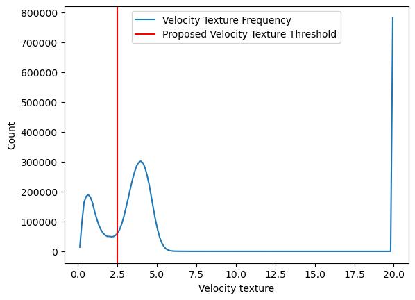

Setup a Gatefilter Object and Apply our Threshold¶

Now we can set up our GateFilter (pyart.filters.GateFilter), which allows us to easily apply masks and filters to our radar object.

gatefilter = pyart.filters.GateFilter(radar)
gatefilter

<pyart.filters.gatefilter.GateFilter at 0x306de0750>

We discovered that a velocity texture threshold of only including values below 3 would be suitable for this dataset, we use the .exclude_above method, specifying we want to exclude texture values above 3.

gatefilter.exclude_above('texture', 2.5)

Plot our Filtered Data¶

Now that we have created a gatefilter, filtering our data using the velocity texture, let’s plot our data!

We need to pass our gatefilter to the plot_ppi_map to apply it to our plot.

# Plot our Unfiltered Data
fig = plt.figure(figsize=[8, 10])
ax = plt.subplot(211, projection=ccrs.PlateCarree())
display = pyart.graph.RadarMapDisplay(radar)
display.plot_ppi_map('mean_doppler_velocity',
                     title='Raw Radial Velocity (no filter)',
                     ax=ax,
                     sweep=1,
                     resolution='50m',
                     vmin=-17,
                     vmax=17,
                     projection=ccrs.PlateCarree(),
                     colorbar_label='Radial Velocity (m/s)',
                     cmap='balance',
                     min_lat=36.3,
                     max_lat=36.9,
                     min_lon=-97.8,
                     max_lon=-97.20)

ax2 = plt.subplot(2,1,2,projection=ccrs.PlateCarree())

# Plot our filtered data
display = pyart.graph.RadarMapDisplay(radar)
display.plot_ppi_map('mean_doppler_velocity',
                     title='Radial Velocity with Velocity Texture Filter',
                     ax=ax2,
                     sweep=1,
                     resolution='50m',
                     vmin=-17,
                     vmax=17, 
                     projection=ccrs.PlateCarree(),
                     colorbar_label='Radial Velocity (m/s)',
                     gatefilter=gatefilter,
                     cmap='balance',
                     min_lat=36.3,
                     max_lat=36.9,
                     min_lon=-97.8,
                     max_lon=-97.20)
plt.show()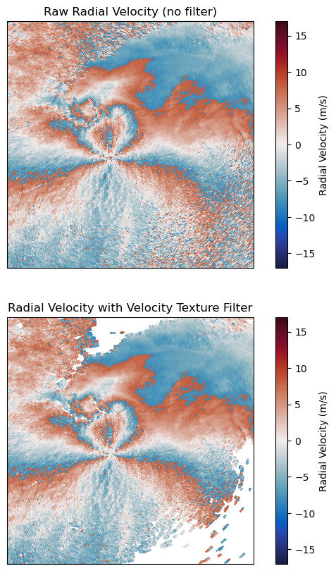

Dealias the Velocity Using the Region-Based Method¶

At this point, we can use the dealias_region_based to dealias the velocities and then add the new field to the radar!

velocity_dealiased = pyart.correct.dealias_region_based(radar,
                                                        vel_field='mean_doppler_velocity',
                                                        nyquist_vel=8.525,
                                                        centered=True,
                                                        gatefilter=gatefilter)

# Add our data dictionary to the radar object
radar.add_field('corrected_velocity', velocity_dealiased, replace_existing=True)

Plot our Cleaned, Dealiased Velocities¶

Plot the new velocities, which now look much more realistic.

fig = plt.figure(figsize=[8, 8])
display = pyart.graph.RadarMapDisplay(radar)
display.plot_ppi_map('corrected_velocity',
                     sweep=1,
                     resolution='50m',
                     vmin=-18,
                     vmax=18, 
                     projection=ccrs.PlateCarree(),
                     colorbar_label='Radial Velocity (m/s)',
                     cmap='balance',
                     gatefilter=gatefilter,
                     min_lat=36.3,
                     max_lat=36.9,
                     min_lon=-97.8,
                     max_lon=-97.20)
plt.show()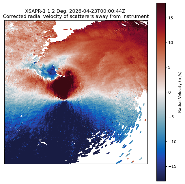

Compare our Raw Velocity Field to our Dealiased, Cleaned Velocity Field¶

As a last comparison, let’s compare our raw, uncorrected velocities with our cleaned velocities, after applying the velocity texture threshold and dealiasing algorithm

# Plot our Unfiltered Data
fig = plt.figure(figsize=[8, 10])
ax = plt.subplot(211, projection=ccrs.PlateCarree())
display = pyart.graph.RadarMapDisplay(radar)
display.plot_ppi_map('mean_doppler_velocity',
                     title='Raw Radial Velocity (no filter)',
                     ax=ax,
                     sweep=1,
                     resolution='50m',
                     vmin=-30,
                     vmax=30,
                     projection=ccrs.PlateCarree(),
                     colorbar_label='Radial Velocity (m/s)',
                     cmap='balance')

ax2 = plt.subplot(2,1,2,projection=ccrs.PlateCarree())

# Plot our filtered, dealiased data
display = pyart.graph.RadarMapDisplay(radar)
display.plot_ppi_map('corrected_velocity',
                     title='Radial Velocity with Velocity Texture Filter and Dealiasing',
                     ax=ax2,
                     sweep=1,
                     resolution='50m',
                     vmin=-30,
                     vmax=30, 
                     projection=ccrs.PlateCarree(),
                     gatefilter=gatefilter,
                     colorbar_label='Radial Velocity (m/s)',
                     cmap='balance')
plt.show()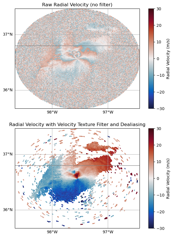

What’s Next¶

In the next notebook, we walk through retrieval development and advanced visualization methods!

References¶

Bharadwaj, N., Hardin, J., Isom, B., Johnson, K., Lindenmaier, I., Matthews, A., Nelson, D., Feng, Y.-C., Wendler, T., Rocque, M., & et al. (2026). X-Band Scanning ARM Precipitation Radar (XSAPRCFR), 2026-04-23 to 2026-04-24, Southern Great Plains (SGP), Deer Creek, OK (Intermediate) (I6). In Atmospheric Radiation Measurement (ARM) user facility. 10.5439/1463663