Snowfall Retrievals CSU X-Band Radar March 14, 2022#
Let’s take a look at precipitation from an event on March 14, 2022 as a part of the SAIL field campaign.
Imports#
import glob
import os
import datetime

import numpy as np
import matplotlib.pyplot as plt
import pyart
import xarray as xr
from matplotlib.dates import DateFormatter
import pandas as pd
import geopandas as gpd
import act
import fiona
Setup Helper Functions#
We setup helper functions to calculate the snowfall retrieval, using following notation:
\(Z = A*S ^ {B}\)
Where:
Z = Reflectivity in dBZ
A = Coefficient applied to Z-S Relationship (not in the exponent)
S = Liquid snowfall rate
B = Coefficient applied to Z-S Relationship (in the exponent)
We also need to apply a snow water equivalent ratio (swe) to convert from liquid to snow (ex. 8 inches of snow –> 1 inch of rain would be 8.0).
This equation now becomes:
\(Z = swe*A*S ^ {B}\)
Solving for S, we get:
\(S = swe * (\frac{z}{a})^{1/B}\)
Where z is reflectivity in units of dB (\(z =10^{Z/10}\))
def snow_rate(radar, swe_ratio, A, B):
    """
    Snow rate applied to a pyart.Radar object

    Takes a given Snow Water Equivilent ratio (swe_ratio), A and B value
    for the Z-S relationship and creates a radar field similar to DBZ
    showing the radar estimated snowfall rate in mm/hr. Then the given
    SWE_ratio, A and B are stored in the radar metadata for later
    reference.

    """
    # Setting up for Z-S relationship:
    snow_z = radar.fields['DBZ']['data'].copy()
    # Convert it from dB to linear units
    z_lin = 10.0**(radar.fields['DBZ']['data']/10.)
    # Apply the Z-S relation.
    snow_z = swe_ratio * (z_lin/A)**(1./B)
    # Add the field back to the radar. Use reflectivity as a template
    radar.add_field_like('DBZ', 'snow_z',  snow_z,
                         replace_existing=True)
    # Update units and metadata
    radar.fields['snow_z']['units'] = 'mm/h'
    radar.fields['snow_z']['standard_name'] = 'snowfall_rate'
    radar.fields['snow_z']['long_name'] = 'snowfall_rate_from_z'
    radar.fields['snow_z']['valid_min'] = 0
    radar.fields['snow_z']['valid_max'] = 500
    radar.fields['snow_z']['swe_ratio'] = swe_ratio
    radar.fields['snow_z']['A'] = A
    radar.fields['snow_z']['B'] = B
    return radar
def snow_rate_from_ds(ds, swe_ratio, A, B, snow_field_name="snow_z", reflectivity_field='DBZ'):
    """
    Snow rate applied to an Xarray.Dataset

    Takes a given Snow Water Equivilent ratio (SWE_ratio), A and B value
    for the Z-S relationship and creates a radar field similar to DBZ
    showing the radar estimated snowfall rate in mm/hr. Then the given
    SWE_ratio, A and B are stored in the radar metadata for later
    reference.
    """
    snow_z = ds[reflectivity_field].copy()

    # Convert it from dB to linear units
    z_lin = 10.0**(snow_z/10.)

    # Apply the Z-S relation.
    snow_z = swe_ratio * (z_lin/A)**(1./B)

    ds[snow_field_name] = snow_z

    field_attrs = {"units": "mm/hr",
                   "standard_name": "snowfall_rate",
                   "long_name":"snowfall_rate_from_z",
                   "valid_min":0,
                   "valid_max":500,
                   "swe_ratio":swe_ratio,
                   "A":A,
                   "B":B}

    ds[snow_field_name].attrs = field_attrs

    return ds
Define the Point Retrievals#
We need to create a set of latitude and longitude values for the different instrumentation locations.
# Define the splash locations [lon,lat]
sail = [-106.987, 38.9586]
kettle_ponds = [-106.9731488, 38.9415427]
brush_creek = [-106.920259, 38.8596282]
avery_point = [-106.9965928, 38.9705885]
pumphouse_site = [-106.9502476, 38.9226741]
roaring_judy = [-106.8530215, 38.7170576]
pluvio = [-106.986, 38.9565]

sites = ["sail", "kettle_ponds", "brush_creek", "avery_point", "pumphouse_site", "roaring_judy", "pluvio"]

# Zip these together!
lons, lats = list(zip(sail,
                      kettle_ponds,
                      brush_creek,
                      avery_point,
                      pumphouse_site,
                      roaring_judy,
                      pluvio))
List the Available Files#
We will use files on the Oak Ridge Laboratory Computing Facility (ORLCF), within the shared SAIL directory /gpfs/wolf/atm124/proj-shared/sail.
These radar files have been merged from a single sweep in each file, to whole volume scans in each file.
file_list = sorted(glob.glob("/gpfs/wolf/atm124/proj-shared/sail/202203_glued/xprecipradar_guc_volume_20220314*"))
file_list[:10]
['/gpfs/wolf/atm124/proj-shared/sail/202203_glued/xprecipradar_guc_volume_20220314-000239.b1.nc',
 '/gpfs/wolf/atm124/proj-shared/sail/202203_glued/xprecipradar_guc_volume_20220314-000759.b1.nc',
 '/gpfs/wolf/atm124/proj-shared/sail/202203_glued/xprecipradar_guc_volume_20220314-001319.b1.nc',
 '/gpfs/wolf/atm124/proj-shared/sail/202203_glued/xprecipradar_guc_volume_20220314-001839.b1.nc',
 '/gpfs/wolf/atm124/proj-shared/sail/202203_glued/xprecipradar_guc_volume_20220314-002359.b1.nc',
 '/gpfs/wolf/atm124/proj-shared/sail/202203_glued/xprecipradar_guc_volume_20220314-002919.b1.nc',
 '/gpfs/wolf/atm124/proj-shared/sail/202203_glued/xprecipradar_guc_volume_20220314-003439.b1.nc',
 '/gpfs/wolf/atm124/proj-shared/sail/202203_glued/xprecipradar_guc_volume_20220314-003959.b1.nc',
 '/gpfs/wolf/atm124/proj-shared/sail/202203_glued/xprecipradar_guc_volume_20220314-004519.b1.nc',
 '/gpfs/wolf/atm124/proj-shared/sail/202203_glued/xprecipradar_guc_volume_20220314-005039.b1.nc']
Read Data + Subset at Points#
def process_point(files, lat, lon):
    """Process data for a single point"""
    ds_all = []
    for file in file_list:
        radar = pyart.io.read(file)
        #-------------------------------------------------------------------------
        # Add in the extra fields to the radar object before extracting the column
        #-------------------------------------------------------------------------
        # Calculate estimated rainfall rate from reflectivty
        #rain = pyart.retrieve.qpe.est_rain_rate_z(radar)
        # Add the estimated rainfall rate back into the radar object
        #radar.add_field('est_rainfall_rate', rain)
        # Call Matt's Z-S function with the constants he used
        radar = snow_rate(radar, 8.5, 28, 1.44)
        #-------------------------------------------------------------------------
        column = pyart.util.columnsect.get_field_location(radar, avery_point[1], avery_point[0])
        # Add a datetime dimension to the xarray radar column
        dt = pd.to_datetime(radar.time["data"], unit='s')[-1]
        coor_ad = column.assign_coords(date=dt.timestamp())
        ncolumn = coor_ad.expand_dims('date')
        # Make sure there are no duplicate height indices
        index = np.unique(column['height'], return_index=True)
        ncolumn = ncolumn.isel(height=index[1])
        # append to the xarray dataset list
        ds_all.append(ncolumn)

    # Combine the xarry DataArrays
    ds = xr.concat(ds_all, 'date')

    # Correct the datetimes
    ds["date"] = pd.to_datetime(ds.date.values, unit='s')

    return ds
def subset_points(file, lats, lons, sites):
    """Subset a radar file for a set of latitudes and longitudes"""

    # Read in the file
    radar = pyart.io.read(file)

    column_list = []
    for lat, lon in zip(lats, lons):
        da = pyart.util.columnsect.get_field_location(radar, lat, lon).interp(height=np.arange(100, 2600, 100))
        da["latitude"], da["longitude"] = lat, lon
        dt = pd.to_datetime(radar.time["data"], unit='s')[-1]
        da.expand_dims("time")
        da["time"] = [dt]
        # Make sure there are no duplicate height indices
        index = np.unique(da['height'], return_index=True)
        ncolumn = da.isel(height=index[1]).dropna(dim='height')
        column_list.append(ncolumn)

    ds = xr.concat(column_list, dim='site')
    ds["site"] = sites
    return ds
Loop through and subset the radar fields at the given points#
%%time
ds_list = []
for file in file_list[:200]:
    ds_list.append(subset_points(file, lats, lons, sites))
/ccsopen/home/mgrover/mgrover/sail-radar-dev/lib/python3.9/site-packages/pyart/core/transforms.py:177: UserWarning: dot_product is larger than one.
  warnings.warn("dot_product is larger than one.")
CPU times: user 9min 41s, sys: 39.4 s, total: 10min 20s
Wall time: 12min
Merge the datasets at the end across time#
ds = xr.concat(ds_list, dim='time')
Apply our Z-S Relationships#
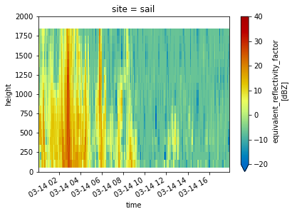
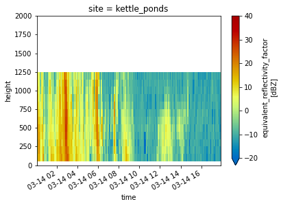
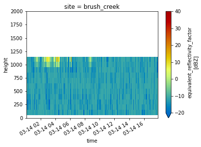
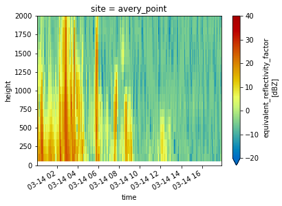
Plot Reflectivity at Each Site#
We loop through and plot reflectivity above each site.
Define our Z-S Relationships#
We start by using the Z-S Relationships Described in Bukovčić et al. (2018), where we refer to following relationships in Table 1:
Source |
Z(S) relation for dry snow |
A Coefficient |
B Coefficient |
Radar Band |
|---|---|---|---|---|
Wolfe and Snider (2012) |
\(Z = {110}S^{2}\) |
110 |
2 |
S |
WSR-88D high plains |
\(Z = {130}S^{2}\) |
130 |
2 |
S |
WSR-88D Intermountain West |
\(Z = {40}S^{2}\) |
40 |
2 |
S |
Matrosov et al.(2009) Braham(1990) |
\(Z = {67}S^{1.28}\) |
67 |
1.28 |
X |
Matrosov et al.(2009) Braham(1990) |
\(Z = {114}S^{1.39}\) |
114 |
1.39 |
X |
Matrosov et al.(2009) Braham(1990) |
\(Z = {136}S^{1.3}\) |
136 |
1.3 |
X |
Matrosov et al.(2009) Braham(1990) |
\(Z = {28}S^{1.44}\) |
28 |
1.44 |
X |
Matrosov et al.(2009) Braham(1990) |
\(Z = {36}S^{1.56}\) |
36 |
1.56 |
X |
Matrosov et al.(2009) Braham(1990) |
\(Z = {48}S^{1.45}\) |
48 |
1.45 |
X |
Matrosov (1992) |
\(Z = {410}S^{1.6}\) |
410 |
1.6 |
X |
Matrosov (1992) |
\(Z = {340}S^{1.6}\) |
340 |
1.75 |
X |
Matrosov (1992) |
\(Z = {240}S^{1.6}\) |
240 |
1.95 |
X |
Boucher and Wieler (1985) |
\(Z = {229}S^{1.65}\) |
229 |
1.65 |
X |
Fujiyoshi et al. (1990) |
\(Z = {427}S^{1.09}\) |
427 |
1.09 |
X |
Puhakka (1975) |
\(Z = {1050}S^{2}\) |
1050 |
2 |
X |
Sekhon and Srivastava (1970) |
\(Z = {1780}S^{2.21}\) |
1780 |
2.21 |
X |
We can plug these into a dictionary for safe keeping.
zs_relationship_dict = {"Wolf_and_Snider":
                        {"A": 110,
                         "B": 2},
                        "WSR_88D_High_Plains":
                        {"A": 130,
                         "B": 2},
                        "WSR_88D_Intermountain_West":
                        {"A": 40,
                         "B": 2},
                        "Matrosov et al.(2009) Braham(1990) 1":
                        {"A": 67,
                         "B": 1.28},
                         "Matrosov et al.(2009) Braham(1990) 2":
                        {"A": 114,
                         "B": 1.39},
                         "Matrosov et al.(2009) Braham(1990) 3":
                        {"A": 136,
                         "B": 1.3},
                         "Matrosov et al.(2009) Braham(1990) 4":
                        {"A": 28,
                         "B": 1.44,},
                         "Matrosov et al.(2009) Braham(1990) 5":
                        {"A": 36,
                         "B": 1.56},
                         "Matrosov et al.(2009) Braham(1990) 6":
                        {"A": 48,
                         "B": 1.45},
                       }
Apply our Z(S) Relationships to the Dataset#
Once we have our dictionary from above, we can apply it to our dataset, using a constant value of a snow liquid water equivalent of 8.5
for relationship in zs_relationship_dict.keys():
    snow_rate_from_ds(ds,
                      8.5,
                      zs_relationship_dict[relationship]["A"],
                      zs_relationship_dict[relationship]["B"],
                      snow_field_name=relationship)
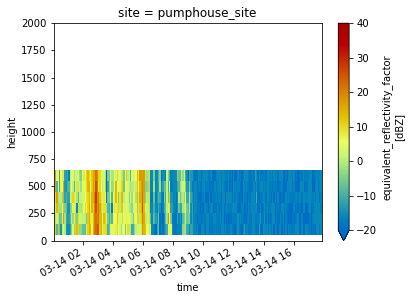
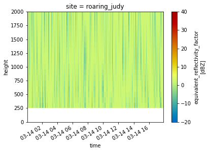
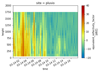
Reflectivity with Height at Each Site#
for site in ds.site:
    ds.sel(site=site).DBZ.plot(x='time',
                             cmap='pyart_HomeyerRainbow',
                             vmin=-20,
                             vmax=40)
    plt.ylim(0, 2000)
    plt.show()
    plt.close()
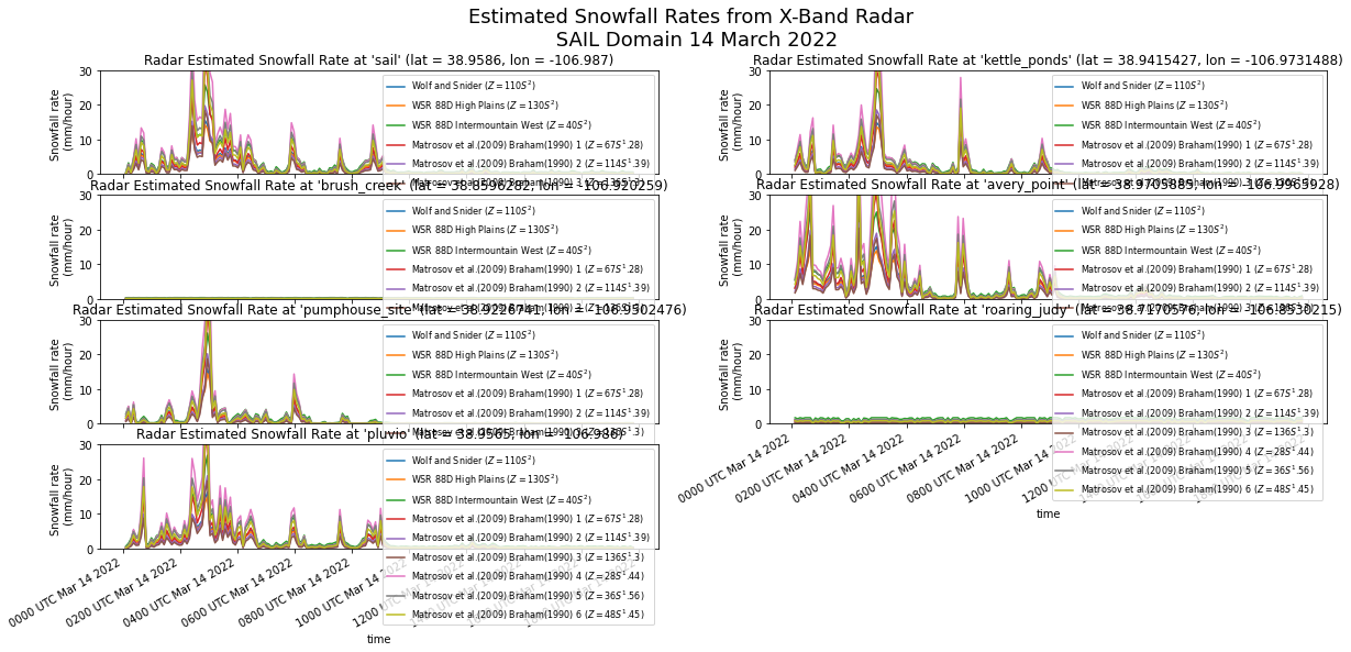
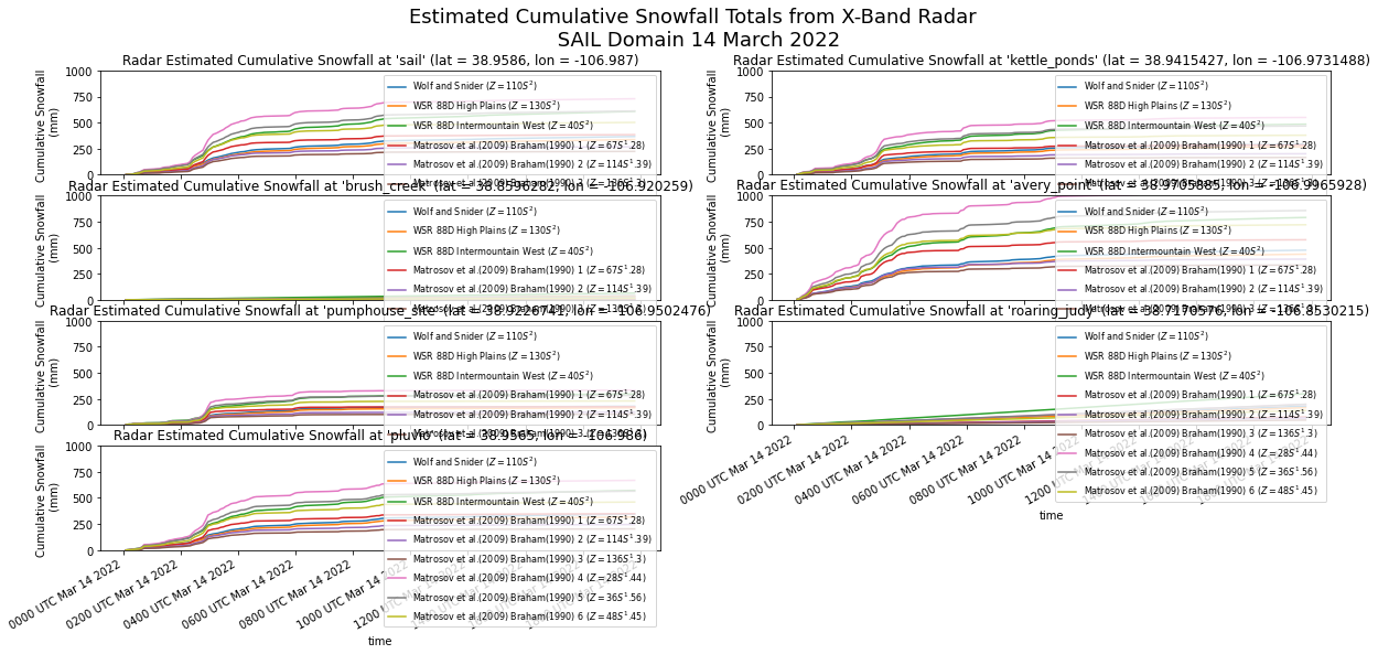
Look at a Timeseries of Snowfall Rates and Totals#
date_form = DateFormatter("%H%M UTC %b %d %Y")
min_value = 0
max_value = 30

fig = plt.figure(figsize=(20,8))

for site in range(len(ds.site.values)):
    ds_at_site = ds.isel(site=site).dropna(dim='height')
    site_name = ds_at_site.site.values
    ax=plt.subplot(int(f"42{site+1}"))
    for relationship in zs_relationship_dict.keys():
        relationship_name = relationship.replace("_", " ")
        a_coefficeint = ds[relationship].A
        b_coefficeint = ds[relationship].B
        relationship_equation = f"$Z = {a_coefficeint}S^{b_coefficeint}$"

        ds_at_site.isel(height=0)[relationship].plot(label=f'{relationship_name} ({relationship_equation})',
                                                     ax=ax)
        ax.xaxis.set_major_formatter(date_form)
        plt.legend(fontsize=8, loc='upper right')

    plt.title(f"Radar Estimated Snowfall Rate at '{site_name}' (lat = {ds_at_site.latitude.values[0]}, lon = {ds_at_site.longitude.values[0]})")

for ax in fig.axes[:-2]:
    ax.axes.axis("tight")
    ax.axes.get_xaxis().set_ticklabels([])
    ax.set_ylabel("Snowfall rate \n (mm/hour)")
    ax.set_xlabel("")
    ax.set_ylim(min_value, max_value)

for ax in fig.axes[-2:]:
    ax.axes.axis("tight")
    ax.set_ylabel("Snowfall rate \n (mm/hour)")
    ax.set_ylim(min_value, max_value)

plt.suptitle("Estimated Snowfall Rates from X-Band Radar \n SAIL Domain 14 March 2022", fontsize=18)
Text(0.5, 0.98, 'Estimated Snowfall Rates from X-Band Radar \n SAIL Domain 14 March 2022')
date_form = DateFormatter("%H%M UTC %b %d %Y")
min_value = 0
max_value = 1000

fig = plt.figure(figsize=(20,8))

for site in range(len(ds.site.values)):
    ds_at_site = ds.isel(site=site).dropna(dim='height')
    site_name = ds_at_site.site.values
    ax=plt.subplot(int(f"42{site+1}"))
    for relationship in zs_relationship_dict.keys():
        relationship_name = relationship.replace("_", " ")
        a_coefficeint = ds[relationship].A
        b_coefficeint = ds[relationship].B
        relationship_equation = f"$Z = {a_coefficeint}S^{b_coefficeint}$"

        ds_at_site.isel(height=0)[relationship].cumsum("time").plot(label=f'{relationship_name} ({relationship_equation})',
                                                                    ax=ax)
        plt.ylim(min_value, max_value)
        ax.xaxis.set_major_formatter(date_form)
        plt.legend(fontsize=8, loc='upper right')

    plt.title(f"Radar Estimated Cumulative Snowfall at '{site_name}' (lat = {ds_at_site.latitude.values[0]}, lon = {ds_at_site.longitude.values[0]})")

for ax in fig.axes[:-2]:
    ax.axes.axis("tight")
    ax.axes.get_xaxis().set_ticklabels([])
    ax.set_ylabel("Cumulative Snowfall \n (mm)")
    ax.set_xlabel("")
    ax.set_ylim(min_value, max_value)

for ax in fig.axes[-2:]:
    ax.axes.axis("tight")
    ax.set_ylabel("Cumulative Snowfall \n (mm)")
    ax.set_ylim(min_value, max_value)

plt.suptitle("Estimated Cumulative Snowfall Totals from X-Band Radar \n SAIL Domain 14 March 2022", fontsize=18)
Text(0.5, 0.98, 'Estimated Cumulative Snowfall Totals from X-Band Radar \n SAIL Domain 14 March 2022')
ds.to_netcdf("sail_snowfall_retrievals_march_14_2022.nc")

