Check Reflectivity Calibration - SAIL X-Band Radar Precipitation

In this example, we walk though how to check the calibration between the X-band and Ka-Band radars

Imports¶

import pyart
import act
import glob
import matplotlib.pyplot as plt
import xarray as xr
from datetime import datetime
from matplotlib.dates import DateFormatter

Download the KAZR data¶

We can access the Ka-band (KAZR) data from the ARM data portal

kazr_files = act.discovery.download_data("mgrover4",
                                         "#############",
                                         "guckazrcfrcorgeM1.c0", 
                                         "2022-03-14",
                                         "2022-03-14")

[DOWNLOADING] guckazrcfrcorgeM1.c0.20220314.000001.nc

We have glued the original xband radar files, and stored these on the local file system in the path below

xprecip_files = sorted(glob.glob("/gpfs/wolf/atm124/proj-shared/sail/202203_glued/xprecipradar_guc_volume_20220314-03*"))

Load in the Data¶

Let’s work with the xarray datasets!

kazr_radar = act.io.read_netcdf(kazr_files)

# this was output from the csu-xband-snowfall-march-14-2022 notebook
xband_ds = xr.open_dataset("sail_snowfall_retrievals_march_14_2022.nc")

We also need to apply the quality flags before working with the kazr data

kazr_lowest_reflectivity = kazr_radar.where(kazr_radar.qc_reflectivity != 1).isel(range=2)[['reflectivity']]

Setup Functions to Calculate Snowfall¶

def snow_rate_from_ds(ds, swe_ratio, A, B, snow_field_name="snow_z", reflectivity_field='DBZ'):
    """
    Snow rate applied to an Xarray.Dataset
    
    Takes a given Snow Water Equivilent ratio (SWE_ratio), A and B value
    for the Z-S relationship and creates a radar field similar to DBZ
    showing the radar estimated snowfall rate in mm/hr. Then the given
    SWE_ratio, A and B are stored in the radar metadata for later 
    reference.   
    """
    snow_z = ds[reflectivity_field].copy()
    
    # Convert it from dB to linear units
    z_lin = 10.0**(snow_z/10.)
    
    # Apply the Z-S relation.
    snow_z = swe_ratio * (z_lin/A)**(1./B)
    
    ds[snow_field_name] = snow_z
    
    field_attrs = {"units": "mm/hr",
                   "standard_name": "snowfall_rate",
                   "long_name":"snowfall_rate_from_z",
                   "valid_min":0,
                   "valid_max":500,
                   "swe_ratio":swe_ratio,
                   "A":A,
                   "B":B}
    
    ds[snow_field_name].attrs = field_attrs
    
    return ds

zs_relationship_dict = {"Wolf_and_Snider":
                        {"A": 110,
                         "B": 2},
                        "WSR_88D_High_Plains":
                        {"A": 130,
                         "B": 2},
                        "WSR_88D_Intermountain_West":
                        {"A": 40,
                         "B": 2},
                        "Matrosov et al.(2009) Braham(1990) 1":
                        {"A": 67,
                         "B": 1.28},
                         "Matrosov et al.(2009) Braham(1990) 2":
                        {"A": 114,
                         "B": 1.39},
                         "Matrosov et al.(2009) Braham(1990) 3":
                        {"A": 136,
                         "B": 1.3},
                         "Matrosov et al.(2009) Braham(1990) 4":
                        {"A": 28,
                         "B": 1.44,},
                         "Matrosov et al.(2009) Braham(1990) 5":
                        {"A": 36,
                         "B": 1.56},
                         "Matrosov et al.(2009) Braham(1990) 6":
                        {"A": 48,
                         "B": 1.45},
                       }

Apply the Z(S) relationships¶

We can now apply our z-s relationships to our dataset

for relationship in zs_relationship_dict.keys():
    snow_rate_from_ds(kazr_lowest_reflectivity,
                      8.5,
                      zs_relationship_dict[relationship]["A"],
                      zs_relationship_dict[relationship]["B"],
                      snow_field_name=relationship,
                      reflectivity_field='reflectivity')

ds = kazr_lowest_reflectivity

Calculate Accumulated Snowfall¶

zs_fields = list(zs_relationship_dict.keys())

ds_resampled = ds.resample(time="1T").mean()

for field in zs_fields:
    ds_resampled[field].attrs["units"] = "mm/hr"
    ds_resampled = act.utils.accumulate_precip(ds_resampled, field)

Plot a Reflectivity Comparison¶

xband_ref = xband_ds.sel(site='pluvio').isel(height=0).DBZ.resample(time='1T').mean().dropna('time')
kaband_ref = ds_resampled.reflectivity

difference = (kaband_ref - xband_ref)

Plot Both Reflectivity Values¶

xband_ref.plot(label='X-Band Reflectivity')
kaband_ref.plot(label='KAZR Reflectivity')
plt.legend()
plt.title('')
plt.xlim('2022-03-14T00', '2022-03-14T09')
plt.savefig("kazr_xband_ref.png", dpi=300)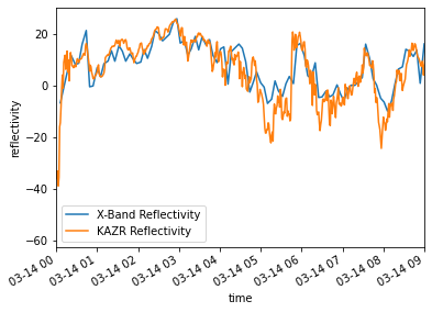

Plot the Difference in Reflectivity¶

difference.plot()
plt.title('KAZR - X-Band Reflectivity')
plt.ylabel('Reflectivity (dB)')
plt.xlim('2022-03-14T00', '2022-03-14T09')
plt.ylim(-20, 20)

(-20.0, 20.0)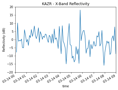

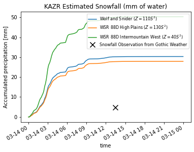
Compare Snowfall Totals with Gothic Weather Station¶

The observation here is from the Gothic wx site, using the liquid precipitation value from March 14, 2022 https://www.gothicwx.org/current-year-data-2022.html

date_form = DateFormatter("%H%M UTC %b %d %Y")

for relationship in list(zs_relationship_dict.keys())[:3]:
    relationship_name = relationship.replace("_", " ")
    a_coefficeint = ds[relationship].A
    b_coefficeint = ds[relationship].B
    relationship_equation = f"$Z = {a_coefficeint}S^{b_coefficeint}$"

    (ds_resampled[relationship+"_accumulated"]).plot(label=f'{relationship_name} ({relationship_equation})')
    ax.xaxis.set_major_formatter(date_form)
    
plt.scatter(datetime(2022, 3, 14, 13, 30),
            4.826,
            c="k",
            s=100,
            marker="x",
            label="Snowfall Observation from Gothic Weather")
    
plt.legend(loc='upper right', fontsize=8)
plt.title("KAZR Estimated Snowfall (mm of water)")
plt.savefig("kazr_snowfall.png", dpi=300)