Exploratory Analysis with Pandas

Exploratory Analysis with Pandas
Overview
- Data Access and Reading
- Understanding the Pandas Data Structure
- Exploratory Data Analysis
Prerequisites
| Concepts | Importance | Notes |
|---|---|---|
| Python Quickstart | Necessary | Intro to dict |
| Numpy Basics | Necessary |
- Time to learn: 30 minutes
Imports
import pandas as pdData Access and Reading
The data for this example/notebook is available from the CSIRO Kennaook/Cape Grim page
https://
More details on the science motivation, data overview, and data citation practices are available on that website. We staged data for you locally in preparation for this workshop - which would be the same as going to the page, downloading, and uploading to this Jupyterhub Space.
Try Reading the Data with Pandas
df = pd.read_csv("../data/CapeGrim_CO2_data_download.csv")---------------------------------------------------------------------------
UnicodeDecodeError Traceback (most recent call last)
Cell In[2], line 1
----> 1 df = pd.read_csv("../data/CapeGrim_CO2_data_download.csv")
File ~/mambaforge/envs/cape-k-student-workshop-2025-dev/lib/python3.12/site-packages/pandas/io/parsers/readers.py:1026, in read_csv(filepath_or_buffer, sep, delimiter, header, names, index_col, usecols, dtype, engine, converters, true_values, false_values, skipinitialspace, skiprows, skipfooter, nrows, na_values, keep_default_na, na_filter, verbose, skip_blank_lines, parse_dates, infer_datetime_format, keep_date_col, date_parser, date_format, dayfirst, cache_dates, iterator, chunksize, compression, thousands, decimal, lineterminator, quotechar, quoting, doublequote, escapechar, comment, encoding, encoding_errors, dialect, on_bad_lines, delim_whitespace, low_memory, memory_map, float_precision, storage_options, dtype_backend)
1013 kwds_defaults = _refine_defaults_read(
1014 dialect,
1015 delimiter,
(...)
1022 dtype_backend=dtype_backend,
1023 )
1024 kwds.update(kwds_defaults)
-> 1026 return _read(filepath_or_buffer, kwds)
File ~/mambaforge/envs/cape-k-student-workshop-2025-dev/lib/python3.12/site-packages/pandas/io/parsers/readers.py:620, in _read(filepath_or_buffer, kwds)
617 _validate_names(kwds.get("names", None))
619 # Create the parser.
--> 620 parser = TextFileReader(filepath_or_buffer, **kwds)
622 if chunksize or iterator:
623 return parser
File ~/mambaforge/envs/cape-k-student-workshop-2025-dev/lib/python3.12/site-packages/pandas/io/parsers/readers.py:1620, in TextFileReader.__init__(self, f, engine, **kwds)
1617 self.options["has_index_names"] = kwds["has_index_names"]
1619 self.handles: IOHandles | None = None
-> 1620 self._engine = self._make_engine(f, self.engine)
File ~/mambaforge/envs/cape-k-student-workshop-2025-dev/lib/python3.12/site-packages/pandas/io/parsers/readers.py:1898, in TextFileReader._make_engine(self, f, engine)
1895 raise ValueError(msg)
1897 try:
-> 1898 return mapping[engine](f, **self.options)
1899 except Exception:
1900 if self.handles is not None:
File ~/mambaforge/envs/cape-k-student-workshop-2025-dev/lib/python3.12/site-packages/pandas/io/parsers/c_parser_wrapper.py:93, in CParserWrapper.__init__(self, src, **kwds)
90 if kwds["dtype_backend"] == "pyarrow":
91 # Fail here loudly instead of in cython after reading
92 import_optional_dependency("pyarrow")
---> 93 self._reader = parsers.TextReader(src, **kwds)
95 self.unnamed_cols = self._reader.unnamed_cols
97 # error: Cannot determine type of 'names'
File parsers.pyx:574, in pandas._libs.parsers.TextReader.__cinit__()
File parsers.pyx:663, in pandas._libs.parsers.TextReader._get_header()
File parsers.pyx:874, in pandas._libs.parsers.TextReader._tokenize_rows()
File parsers.pyx:891, in pandas._libs.parsers.TextReader._check_tokenize_status()
File parsers.pyx:2053, in pandas._libs.parsers.raise_parser_error()
File <frozen codecs>:322, in decode(self, input, final)
UnicodeDecodeError: 'utf-8' codec can't decode byte 0x91 in position 38419: invalid start byteTroubleshooting the Data Reading
By default, we cannot read the data! We need to pass more information to pandas to be able to read the data. For example, if we open the file with a text reader, we notice there is a good amount of metadata at the top of the file
Metadata: Data about our data. This provides helpful links, when data was processed, and units. All of this data is critical to understanding our data before we perform analysis.
df = pd.read_csv("../data/CapeGrim_CO2_data_download.csv",
                 skiprows=24, # the number of rows at the top of the file with metadata
                 skipfooter=70, # the number of rows at the bottom of the file with metadata
                 encoding = "ISO-8859-1") # there are some special characters - we need a specific encoding
dfUnderstanding the Pandas Data Structure
The pandas DataFrame...
...is a labeled, two-dimensional columnar structure, similar to a table, spreadsheet, or the R data.frame.

The columns that make up our DataFrame can be lists, dictionaries, NumPy arrays, pandas Series, or many other data types not mentioned here. Within these columns, you can have data values of many different data types used in Python and NumPy, including text, numbers, and dates/times. The first column of a DataFrame, shown in the image above in dark gray, is uniquely referred to as an index; this column contains information characterizing each row of our DataFrame. Similar to any other column, the index can label rows by text, numbers, datetime objects, and many other data types. Datetime objects are a quite popular way to label rows.
For our first example using Pandas DataFrames, we start by reading in some data in comma-separated value (.csv) format. We retrieve this dataset from our local data directory; however, the dataset was originally contained within the CSIRO data page. This dataset contains many types of greenhouse gas data, including gas measurements at Kennaook/Cape Grim. For more information on this dataset, review the description here.
df.indexRangeIndex(start=0, stop=584, step=1)The DataFrame index, as described above, contains information characterizing rows; each row has a unique ID value, which is displayed in the index column. By default, the IDs for rows in a DataFrame are represented as sequential integers, which start at 0.
At the moment, the index column of our DataFrame is not very helpful for humans. However, Pandas has clever ways to make index columns more human-readable. The next example demonstrates how to use optional keyword arguments to convert DataFrame index IDs to a human-friendly datetime format.
df = pd.read_csv("../data/CapeGrim_CO2_data_download.csv",
                 skiprows=24, # the number of rows at the top of the file with metadata
                 skipfooter=70, # the number of rows at the bottom of the file with metadata
                 encoding = "ISO-8859-1", # there are some special characters - we need a specific encoding
                 parse_dates={"date":["MM", "DD", "YYYY"]}, # parse the date columns
                 engine="python", # make sure we use the python engine
                 index_col=0)
dfEach of our data rows is now helpfully labeled by a datetime-object-like index value; this means that we can now easily identify data values not only by named columns, but also by date labels on rows. This is a sneak preview of the DatetimeIndex functionality of Pandas; this functionality enables a large portion of Pandas’ timeseries-related usage. Don’t worry; DatetimeIndex will be discussed in full detail later on this page. In the meantime, let’s look at the columns of data read in from the .csv file:
df.columnsIndex(['DATE', 'CO2(ppm)', 'SD(ppm)', 'GR(ppm/yr)', 'Source'], dtype='object')The pandas Series...
...is essentially any one of the columns of our DataFrame. A Series also includes the index column from the source DataFrame, in order to provide a label for each value in the Series.

The pandas Series is a fast and capable 1-dimensional array of nearly any data type we could want, and it can behave very similarly to a NumPy ndarray or a Python dict. You can take a look at any of the Series that make up your DataFrame, either by using its column name and the Python dict notation, or by using dot-shorthand with the column name:
df["CO2(ppm)"]date
1976-05-15 328.861
1976-06-15 328.988
1976-07-15 329.653
1976-08-15 330.550
1976-09-15 330.872
...
2024-08-15 420.795
2024-09-15 421.180
2024-10-15 421.397
2024-11-15 421.414
2024-12-15 421.377
Name: CO2(ppm), Length: 584, dtype: float64Slicing and Dicing the DataFrame and Series
In this section, we will expand on topics covered in the previous sections on this page. One of the most important concepts to learn about Pandas is that it allows you to access anything by its associated label, regardless of data organization structure.
Indexing a Series
As a review of previous examples, we’ll start our next example by pulling a Series out of our DataFrame using its column label.
co2_series = df["CO2(ppm)"]

co2_series
date
1976-05-15 328.861
1976-06-15 328.988
1976-07-15 329.653
1976-08-15 330.550
1976-09-15 330.872
...
2024-08-15 420.795
2024-09-15 421.180
2024-10-15 421.397
2024-11-15 421.414
2024-12-15 421.377
Name: CO2(ppm), Length: 584, dtype: float64You can use syntax similar to that of NumPy ndarrays to index, select, and subset with Pandas Series, as shown in this example:
co2_series["1982-01-01":"1982-12-01"]date
1982-01-15 337.306
1982-02-15 337.127
1982-03-15 337.274
1982-04-15 337.698
1982-05-15 338.032
1982-06-15 338.186
1982-07-15 338.551
1982-08-15 338.898
1982-09-15 338.822
1982-10-15 338.634
1982-11-15 338.557
Name: CO2(ppm), dtype: float64This is an example of label-based slicing. With label-based slicing, Pandas will automatically find a range of values based on the labels you specify.
Info
As opposed to index-based slices, label-based slices are inclusive of the final value.If you already have some knowledge of xarray (used with ACT), you will quite likely know how to create slice objects by hand. This can also be used in pandas, as shown below. If you are completely unfamiliar with xarray, it will be covered on a later Pythia tutorial page.
co2_series[slice("1982-01-01", "1982-12-01")]date
1982-01-15 337.306
1982-02-15 337.127
1982-03-15 337.274
1982-04-15 337.698
1982-05-15 338.032
1982-06-15 338.186
1982-07-15 338.551
1982-08-15 338.898
1982-09-15 338.822
1982-10-15 338.634
1982-11-15 338.557
Name: CO2(ppm), dtype: float64Using .iloc and .loc to index
In this section, we introduce ways to access data that are preferred by Pandas over the methods listed above. When accessing by label, it is preferred to use the .loc method, and when accessing by index, the .iloc method is preferred. These methods behave similarly to the notation introduced above, but provide more speed, security, and rigor in your value selection. Using these methods can also help you avoid chained assignment warnings generated by pandas.
co2_series.iloc[3]np.float64(330.55)co2_series.iloc[0:12]date
1976-05-15 328.861
1976-06-15 328.988
1976-07-15 329.653
1976-08-15 330.550
1976-09-15 330.872
1976-10-15 330.899
1976-11-15 330.883
1976-12-15 330.677
1977-01-15 330.529
1977-02-15 330.543
1977-03-15 330.724
1977-04-15 330.805
Name: CO2(ppm), dtype: float64co2_series.loc["1976-05-15"]np.float64(328.861)co2_series.loc["1977-01-01":"1977-12-31"]date
1977-01-15 330.529
1977-02-15 330.543
1977-03-15 330.724
1977-04-15 330.805
1977-05-15 331.007
1977-06-15 331.500
1977-07-15 331.800
1977-08-15 332.327
1977-09-15 332.940
1977-10-15 333.034
1977-11-15 332.778
1977-12-15 332.377
Name: CO2(ppm), dtype: float64Extending to the DataFrame
These subsetting capabilities can also be used in a full DataFrame; however, if you use the same syntax, there are issues, as shown below:
df["1977-01-01"]---------------------------------------------------------------------------
KeyError Traceback (most recent call last)
File ~/mambaforge/envs/cape-k-student-workshop-2025-dev/lib/python3.12/site-packages/pandas/core/indexes/base.py:3805, in Index.get_loc(self, key)
3804 try:
-> 3805 return self._engine.get_loc(casted_key)
3806 except KeyError as err:
File index.pyx:167, in pandas._libs.index.IndexEngine.get_loc()
File index.pyx:196, in pandas._libs.index.IndexEngine.get_loc()
File pandas/_libs/hashtable_class_helper.pxi:7081, in pandas._libs.hashtable.PyObjectHashTable.get_item()
File pandas/_libs/hashtable_class_helper.pxi:7089, in pandas._libs.hashtable.PyObjectHashTable.get_item()
KeyError: '1977-01-01'
The above exception was the direct cause of the following exception:
KeyError Traceback (most recent call last)
Cell In[15], line 1
----> 1 df["1977-01-01"]
File ~/mambaforge/envs/cape-k-student-workshop-2025-dev/lib/python3.12/site-packages/pandas/core/frame.py:4102, in DataFrame.__getitem__(self, key)
4100 if self.columns.nlevels > 1:
4101 return self._getitem_multilevel(key)
-> 4102 indexer = self.columns.get_loc(key)
4103 if is_integer(indexer):
4104 indexer = [indexer]
File ~/mambaforge/envs/cape-k-student-workshop-2025-dev/lib/python3.12/site-packages/pandas/core/indexes/base.py:3812, in Index.get_loc(self, key)
3807 if isinstance(casted_key, slice) or (
3808 isinstance(casted_key, abc.Iterable)
3809 and any(isinstance(x, slice) for x in casted_key)
3810 ):
3811 raise InvalidIndexError(key)
-> 3812 raise KeyError(key) from err
3813 except TypeError:
3814 # If we have a listlike key, _check_indexing_error will raise
3815 # InvalidIndexError. Otherwise we fall through and re-raise
3816 # the TypeError.
3817 self._check_indexing_error(key)
KeyError: '1977-01-01'Danger
Attempting to useSeries subsetting with a DataFrame can crash your program. A proper way to subset a DataFrame is shown below.When indexing a DataFrame, pandas will not assume as readily the intention of your code. In this case, using a row label by itself will not work; with DataFrames, labels are used for identifying columns.
df["CO2(ppm)"]As shown below, you also cannot subset columns in a DataFrame using integer indices:
df[0]---------------------------------------------------------------------------
KeyError Traceback (most recent call last)
File ~/mambaforge/envs/cape-k-student-workshop-2025-dev/lib/python3.12/site-packages/pandas/core/indexes/base.py:3805, in Index.get_loc(self, key)
3804 try:
-> 3805 return self._engine.get_loc(casted_key)
3806 except KeyError as err:
File index.pyx:167, in pandas._libs.index.IndexEngine.get_loc()
File index.pyx:196, in pandas._libs.index.IndexEngine.get_loc()
File pandas/_libs/hashtable_class_helper.pxi:7081, in pandas._libs.hashtable.PyObjectHashTable.get_item()
File pandas/_libs/hashtable_class_helper.pxi:7089, in pandas._libs.hashtable.PyObjectHashTable.get_item()
KeyError: 0
The above exception was the direct cause of the following exception:
KeyError Traceback (most recent call last)
Cell In[16], line 1
----> 1 df[0]
File ~/mambaforge/envs/cape-k-student-workshop-2025-dev/lib/python3.12/site-packages/pandas/core/frame.py:4102, in DataFrame.__getitem__(self, key)
4100 if self.columns.nlevels > 1:
4101 return self._getitem_multilevel(key)
-> 4102 indexer = self.columns.get_loc(key)
4103 if is_integer(indexer):
4104 indexer = [indexer]
File ~/mambaforge/envs/cape-k-student-workshop-2025-dev/lib/python3.12/site-packages/pandas/core/indexes/base.py:3812, in Index.get_loc(self, key)
3807 if isinstance(casted_key, slice) or (
3808 isinstance(casted_key, abc.Iterable)
3809 and any(isinstance(x, slice) for x in casted_key)
3810 ):
3811 raise InvalidIndexError(key)
-> 3812 raise KeyError(key) from err
3813 except TypeError:
3814 # If we have a listlike key, _check_indexing_error will raise
3815 # InvalidIndexError. Otherwise we fall through and re-raise
3816 # the TypeError.
3817 self._check_indexing_error(key)
KeyError: 0From earlier examples, we know that we can use an index or label with a DataFrame to pull out a column as a Series, and we know that we can use an index or label with a Series to pull out a single value. Therefore, by chaining brackets, we can pull any individual data value out of the DataFrame.
df["CO2(ppm)"]["1982-04-15"]np.float64(337.698)df["CO2(ppm)"][71]/var/folders/bw/c9j8z20x45s2y20vv6528qjc0000gq/T/ipykernel_85673/1011012163.py:1: FutureWarning: Series.__getitem__ treating keys as positions is deprecated. In a future version, integer keys will always be treated as labels (consistent with DataFrame behavior). To access a value by position, use `ser.iloc[pos]`
df["CO2(ppm)"][71]
np.float64(337.698)However, subsetting data using this chained-bracket technique is not preferred by Pandas. As described above, Pandas prefers us to use the .loc and .iloc methods for subsetting. In addition, these methods provide a clearer, more efficient way to extract specific data from a DataFrame, as illustrated below:
df.loc["1982-04-15", "CO2(ppm)"]np.float64(337.698)Info
When using this syntax to pull individual data values from a DataFrame, make sure to list the row first, and then the column.The .loc and .iloc methods also allow us to pull entire rows out of a DataFrame, as shown in these examples:
df.loc["1982-04-15"]DATE 1982.2849
CO2(ppm) 337.698
SD(ppm) 0.241
GR(ppm/yr) 0.562012
Source in situ
Name: 1982-04-15 00:00:00, dtype: objectdf.loc["1982-01-01":"1982-12-01"]df.iloc[3]DATE 1976.6202
CO2(ppm) 330.55
SD(ppm) 0.201
GR(ppm/yr) NaN
Source in situ
Name: 1976-08-15 00:00:00, dtype: objectdf.iloc[0:12]In the next example, we illustrate how you can use slices of rows and lists of columns to create a smaller DataFrame out of an existing DataFrame:
df.loc[
    "1982-01-01":"1982-12-01",  # slice of rows
    ["CO2(ppm)", "SD(ppm)"],  # list of columns
]Info
There are certain limitations to these subsetting techniques. For more information on these limitations, as well as a comparison ofDataFrame and Series indexing methods, see the Pandas indexing documentation.Exploratory Data Analysis
Get a Quick Look at the Beginning/End of your DataFrame
Pandas also gives you a few shortcuts to quickly investigate entire DataFrames. The head method shows the first five rows of a DataFrame, and the tail method shows the last five rows of a DataFrame.
df.head()df.tail()Quick Plots of Your Data
A good way to explore your data is by making a simple plot. Pandas contains its own plot method; this allows us to plot Pandas series without needing matplotlib. In this example, we plot the Nino34 series of our df DataFrame in this way:
df["CO2(ppm)"].plot();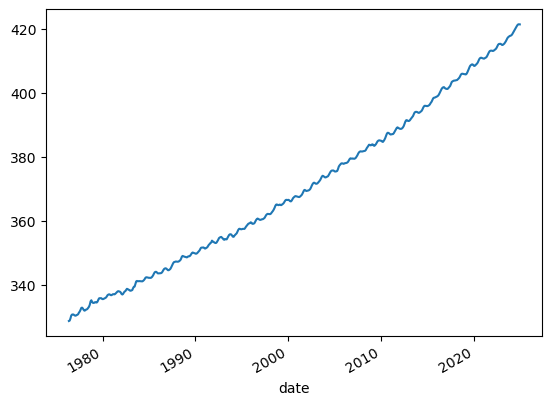
Before, we called .plot(), which generated a single line plot. Line plots can be helpful for understanding some types of data, but there are other types of data that can be better understood with different plot types. For example, if your data values form a distribution, you can better understand them using a histogram plot.
The code for plotting histogram data differs in two ways from the code above for the line plot. First, two series are being used from the DataFrame instead of one. Second, after calling the plot method, we call an additional method called hist, which converts the plot into a histogram.
df[['CO2(ppm)']].plot.hist();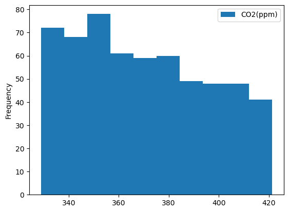
The histogram plot helped us better understand our data; there are clear differences in the distributions. To even better understand this type of data, it may also be helpful to create a box plot. This can be done using the same line of code, with one change: we call the box method instead of hist.
df[['CO2(ppm)']].plot.box();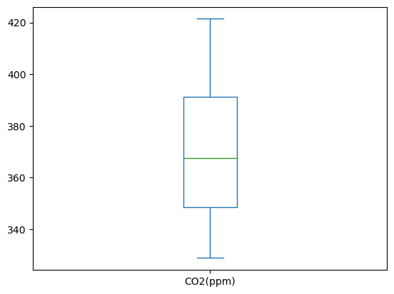
Just like the histogram plot, this box plot indicates a clear difference in the distributions. Using multiple types of plot in this way can be useful for verifying large datasets. The pandas plotting methods are capable of creating many different types of plots. To see how to use the plotting methods to generate each type of plot, please review the pandas plot documentation.
Customize your Plot
The pandas plotting methods are, in fact, wrappers for similar methods in matplotlib. This means that you can customize pandas plots by including keyword arguments to the plotting methods. These keyword arguments, for the most part, are equivalent to their matplotlib counterparts.
df['CO2(ppm)'].plot(
    color='black', # Change the color
    linewidth=2, # Make the line wider
    xlabel='Year', # Add a label to the xaxis
    ylabel=f'$CO^{2}$ [ppm]', # Add a label to the axis including units and latex syntax
    figsize=(8, 6), # Change the dimensions of the figure
);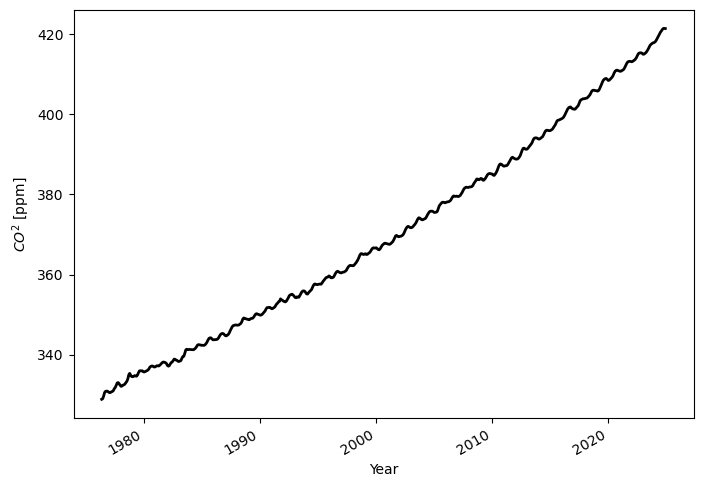
Although plotting data can provide a clear visual picture of data values, sometimes a more quantitative look at data is warranted. As elaborated on in the next section, this can be achieved using the describe method. The describe method is called on the entire DataFrame, and returns various summarized statistics for each column in the DataFrame.
Basic Statistics
We can garner statistics for a DataFrame by using the describe method. When this method is called on a DataFrame, a set of statistics is returned in tabular format. The columns match those of the DataFrame, and the rows indicate different statistics, such as minimum.
df.describe()You can also view specific statistics using corresponding methods. In this example, we look at the mean values in the entire DataFrame, using the mean method. When such methods are called on the entire DataFrame, a Series is returned. The indices of this Series are the column names in the DataFrame, and the values are the calculated values (in this case, mean values) for the DataFrame columns.
df["CO2(ppm)"].mean()np.float64(370.29387157534245)Subsetting Using the Datetime Column
Slicing is a useful technique for subsetting a DataFrame, but there are also other options that can be equally useful. In this section, some of these additional techniques are covered.
If your DataFrame uses datetime values for indices, you can select data from only one month using df.index.month. In this example, we specify the number 1, which only selects data from January.
This example shows how to create a new column containing the month portion of the datetime index for each data row. The value returned by df.index.month is used to obtain the data for this new column:
df['month'] = df.index.monthThis next example illustrates how to use the new month column to calculate average monthly values over the other data columns. First, we use the groupby method to group the other columns by the month. Second, we take the average (mean) to obtain the monthly averages. Finally, we plot the resulting data as a line plot by simply calling plot().
df.groupby('month')["CO2(ppm)"].mean().plot();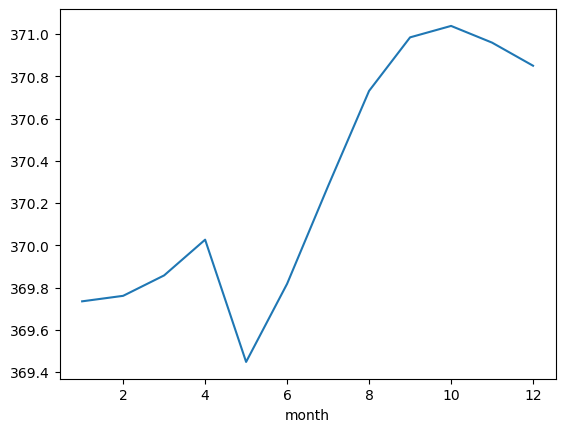
Investigating Extreme Values
If you need to search for rows that meet a specific criterion, you can use conditional indexing. In this example, we search for rows where the values exceed the 95th percentile across all the data from the beginning of the record:
percentile_95 = df["CO2(ppm)"].quantile(.95) # Calculate the 95th percentile
df[df["CO2(ppm)"] > percentile_95] # Filter the data for greater than the 95th percentileThis example shows how to use the sort_values method on a DataFrame. This method sorts values in a DataFrame by the column specified as an argument.
df.sort_values('CO2(ppm)')You can also reverse the ordering of the sort by specifying the ascending keyword argument as False:
df.sort_values('CO2(ppm)', ascending=False)Resampling
In these examples, we illustrate a process known as resampling. Using resampling, you can change the frequency of index data values, reducing so-called ‘noise’ in a data plot. This is especially useful when working with timeseries data; plots can be equally effective with resampled data in these cases. The resampling performed in these examples converts monthly values to yearly averages. This is performed by passing the value ‘1YE’ to the resample method.
df['CO2(ppm)'].resample('1YE').mean().plot();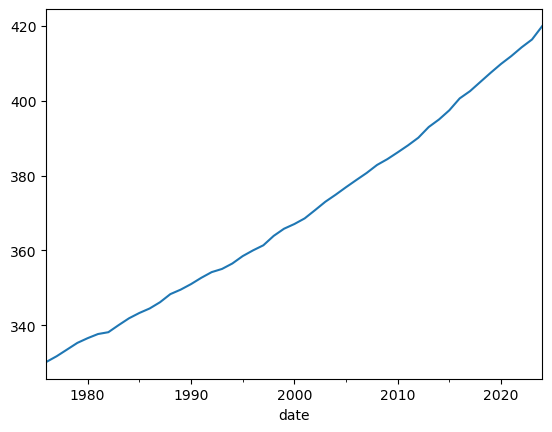
Applying operations to a DataFrame
One of the most commonly used features in Pandas is the performing of calculations to multiple data values in a DataFrame simultaneously. Let’s first look at a familiar concept: a function that converts single values. The following example uses such a function to convert concentrations from parts ber million (ppm) to parts per billion (ppb):
def convert_ppm_to_ppb(concentration_ppm):
    """
    Converts from parts per million to parts per billion
    """

    return concentration_ppm * 1000
# Convert a single value
convert_ppm_to_ppb(1)1000The following examples instead illustrate a new concept: using such functions with DataFrames and Series. For the first example, we start by creating a Series; in order to do so, we subset the DataFrame by the CO2(ppm) column. This has already been done earlier in this page; we do not need to create this Series again. We are using this particular Series for a reason: the data values are in parts per million.
co2_seriesdate
1976-05-15 328.861
1976-06-15 328.988
1976-07-15 329.653
1976-08-15 330.550
1976-09-15 330.872
...
2024-08-15 420.795
2024-09-15 421.180
2024-10-15 421.397
2024-11-15 421.414
2024-12-15 421.377
Name: CO2(ppm), Length: 584, dtype: float64This example illustrates how to use the temperature-conversion function defined above on a Series object. Just as calling the function with a single value returns a single value, calling the function on a Series object returns another Series object. The function performs the temperature conversion on each data value in the Series, and returns a Series with all values converted.
convert_ppm_to_ppb(co2_series)date
1976-05-15 328861.0
1976-06-15 328988.0
1976-07-15 329653.0
1976-08-15 330550.0
1976-09-15 330872.0
...
2024-08-15 420795.0
2024-09-15 421180.0
2024-10-15 421397.0
2024-11-15 421414.0
2024-12-15 421377.0
Name: CO2(ppm), Length: 584, dtype: float64If we call the .values method on the Series passed to the function, the Series is converted to a numpy array, as described above. The function then converts each value in the numpy array, and returns a new numpy array with all values sorted.
Warning
It is recommended to only convertSeries to NumPy arrays when necessary; doing so removes the label information that enables much of the Pandas core functionality.convert_ppm_to_ppb(co2_series.values)array([328861., 328988., 329653., 330550., 330872., 330899., 330883.,
330677., 330529., 330543., 330724., 330805., 331007., 331500.,
331800., 332327., 332940., 333034., 332778., 332377., 332094.,
332175., 332398., 332474., 332646., 333015., 333317., 333926.,
334977., 335333., 334826., 334531., 334498., 334585., 334763.,
334703., 334626., 334889., 335452., 335936., 335981., 335979.,
335971., 335733., 335678., 335778., 335898., 336057., 336185.,
336532., 336930., 337096., 337190., 337116., 336938., 336916.,
337089., 337230., 337226., 337174., 337346., 337587., 337832.,
338093., 338165., 338072., 338000., 337768., 337306., 337127.,
337274., 337698., 338032., 338186., 338551., 338898., 338822.,
338634., 338557., 338328., 338307., 338427., 338519., 339115.,
339532., 339601., 340338., 341204., 341354., 341257., 341296.,
341307., 341273., 341271., 341242., 341232., 341390., 341620.,
341935., 342359., 342508., 342472., 342426., 342342., 342329.,
342289., 342319., 342488., 342768., 343159., 343656., 344069.,
344197., 344195., 343945., 343710., 343715., 343741., 343765.,
343784., 343917., 344236., 344685., 345057., 345237., 345307.,
345205., 344955., 344717., 344702., 344858., 345053., 345442.,
346005., 346472., 346965., 347257., 347303., 347406., 347405.,
347357., 347368., 347428., 347607., 347812., 348252., 348912.,
349156., 349051., 348948., 348872., 348832., 348717., 348756.,
348976., 349056., 349065., 349297., 349682., 350047., 350222.,
350147., 350072., 349966., 349849., 349894., 350055., 350350.,
350612., 350892., 351374., 351736., 351773., 351784., 351808.,
351614., 351454., 351551., 351705., 351879., 352283., 352654.,
352860., 353191., 353328., 353925., 353679., 353567., 353356.,
353235., 353170., 353356., 353733., 354173., 354695., 354897.,
355029., 355083., 354862., 354606., 354278., 354203., 354423.,
354358., 354326., 354763., 355237., 355656., 355882., 355923.,
355828., 355517., 355152., 355132., 355454., 355741., 355962.,
356230., 356716., 357281., 357606., 357625., 357507., 357472.,
357535., 357610., 357600., 357588., 357891., 358293., 358580.,
358916., 359199., 359310., 359381., 359643., 359537., 359193.,
359188., 359234., 359422., 359914., 360339., 360675., 360815.,
360685., 360534., 360407., 360424., 360546., 360591., 360654.,
360817., 361026., 361423., 361885., 362148., 362282., 362257.,
362205., 362182., 362320., 362617., 362895., 363258., 363684.,
364198., 364816., 365188., 365204., 365074., 364992., 365126.,
365177., 364993., 365050., 365286., 365438., 365726., 366161.,
366522., 366670., 366609., 366619., 366665., 366468., 366238.,
366171., 366388., 366839., 367242., 367486., 367706., 367827.,
367756., 367663., 367606., 367547., 367537., 367701., 367931.,
368176., 368586., 369133., 369631., 369760., 369559., 369413.,
369481., 369544., 369601., 369763., 370011., 370477., 371049.,
371539., 371878., 372010., 371896., 371706., 371674., 371752.,
371954., 372235., 372521., 372865., 373325., 373860., 374156.,
374079., 373862., 373680., 373647., 373776., 373869., 374021.,
374415., 374896., 375298., 375639., 375795., 375817., 375812.,
375632., 375477., 375522., 375553., 375688., 376289., 377049.,
377418., 377703., 377979., 378053., 377999., 377886., 377972.,
378104., 378120., 378180., 378303., 378537., 378929., 379381.,
379604., 379534., 379491., 379566., 379492., 379459., 379568.,
379766., 380139., 380527., 381033., 381451., 381660., 381786.,
381764., 381718., 381779., 381859., 381867., 381961., 382229.,
382729., 383071., 383434., 383839., 383796., 383645., 383723.,
383962., 383925., 383598., 383502., 383728., 384019., 384418.,
384884., 385100., 385212., 385190., 385108., 385072., 384815.,
384720., 385016., 385399., 385904., 386568., 387212., 387560.,
387555., 387408., 387166., 387018., 387090., 387147., 387156.,
387403., 387833., 388198., 388634., 389129., 389260., 389072.,
388944., 388817., 388789., 388827., 388999., 389287., 389713.,
390377., 391050., 391480., 391518., 391319., 391238., 391298.,
391526., 391859., 392160., 392465., 392806., 393387., 393891.,
394075., 394102., 394076., 393945., 393791., 393818., 394003.,
394208., 394378., 394788., 395339., 395777., 396002., 395992.,
395948., 395889., 395922., 396062., 396203., 396527., 396943.,
397260., 397755., 398314., 398507., 398542., 398663., 398776.,
398902., 399073., 399333., 399782., 400294., 400802., 401288.,
401589., 401765., 401803., 401542., 401349., 401284., 401228.,
401316., 401597., 401873., 402182., 402821., 403405., 403616.,
403748., 403860., 403858., 403919., 403979., 404036., 404260.,
404518., 404817., 405305., 405770., 405970., 405993., 405918.,
405872., 405843., 405758., 405895., 406308., 406847., 407432.,
408038., 408504., 408728., 408886., 408906., 408670., 408418.,
408494., 408750., 408984., 409236., 409660., 410236., 410700.,
410922., 410995., 410904., 410787., 410719., 410718., 410876.,
411005., 411197., 411617., 412127., 412633., 413017., 413156.,
413192., 413170., 413086., 413148., 413327., 413488., 413716.,
414068., 414547., 415053., 415279., 415304., 415329., 415190.,
414958., 414989., 415174., 415379., 415713., 416113., 416556.,
417083., 417393., 417575., 417774., 417840., 417971., 418228.,
418608., 419073., 419514., 420034., 420463., 420795., 421180.,
421397., 421414., 421377.])As described above, when our temperature-conversion function accepts a Series as an argument, it returns a Series. We can directly assign this returned Series to a new column in our DataFrame, as shown below:
df['CO2(ppb)'] =convert_ppm_to_ppb(co2_series)
df['CO2(ppb)']
date
1976-05-15 328861.0
1976-06-15 328988.0
1976-07-15 329653.0
1976-08-15 330550.0
1976-09-15 330872.0
...
2024-08-15 420795.0
2024-09-15 421180.0
2024-10-15 421397.0
2024-11-15 421414.0
2024-12-15 421377.0
Name: CO2(ppb), Length: 584, dtype: float64In this final example, we demonstrate the use of the to_csv method to save a DataFrame as a .csv file. This example also demonstrates the read_csv method, which reads .csv files into Pandas DataFrames.
df.to_csv("CapeGrim_CO2_data_analyzed.csv")pd.read_csv('CapeGrim_CO2_data_analyzed.csv', index_col=0, parse_dates=True)Summary
- Pandas is a very powerful tool for working with tabular (i.e., spreadsheet-style) data
- There are multiple ways of subsetting your pandas dataframe or series
- Pandas allows you to refer to subsets of data by label, which generally makes code more readable and more robust
- Pandas can be helpful for exploratory data analysis, including plotting and basic statistics
- One can apply calculations to pandas dataframes and save the output via
csvfiles
What’s Next?
In the next notebook, we will take a look at how to work with cloud radar/remote sensing data.