Project Pythia Logo

Exploration of CSAPR-2 Z-R relationships over BNF¶

Overview¶

This notebook explores the relationship between radar reflectivity (Z) and rain rate (R) CSAPR2 radar over BNF. Accuracy of ZR relationship is affected by the variability of raindrop size distributions (DSDs). Rainfall also causes attenuation of radar signals, particularly at higher frequencies. This can also be used for rainfall estimation. The LDQUANTS is a laser disdrometer based product from ARM that characterizes DSD. We want to optimized the Z-R relationship over BNF, for more accurate rainfall estimations compared to using generalized or default Z-R relationships. This notebook will demonstrate the derivation of both Z-R and k-R (attenuation-rain rate) relationships using LDQUANTS data.

Prerequisites¶

Concepts	Importance	Notes
Linear Regression	Necessary
Radar Reflectivity	Necessary
Understanding of NetCDF	Helpful	Familiarity with metadata structure

Time to learn: 30 min.
System requirements:
- Populate with any system, version, or non-Python software requirements if necessary
- Otherwise use the concepts table above and the Imports section below to describe required packages as necessary
- If no extra requirements, remove the System requirements point altogether

Z-R and k-R Relationships from LDQUANTS for BNF M1¶

The notebook presents an analysis to derive empirical relationships between radar reflectivity (dBZ) and rain rate (R), and also specific attenuation (k) and R using Drop Size Distribution (DSD) from LDQUANTS from NetCDF files.

imports and file reading¶

import xarray as xr
import numpy as np
import matplotlib.pyplot as plt
import seaborn as sns

import glob

file_dir = '/Users/bhupendra/projects/bnf-amf3/data/bnfldquantsM1.c1/' 
file_pattern = 'bnfldquantsM1.c1.2025*.nc' 
file_paths = sorted(glob.glob(file_dir + file_pattern)) 

print(len(file_paths))

I will use xarray to read mutiple files

ds = xr.open_mfdataset(file_paths, combine='by_coords')
print(ds)

<xarray.Dataset> Size: 10MB
Dimensions:                                      (time: 54412)
Coordinates:
  * time                                         (time) datetime64[ns] 435kB ...
Data variables: (12/42)
    base_time                                    (time) datetime64[ns] 435kB ...
    time_offset                                  (time) datetime64[ns] 435kB dask.array<chunksize=(1440,), meta=np.ndarray>
    rain_rate                                    (time) float32 218kB dask.array<chunksize=(1440,), meta=np.ndarray>
    reflectivity_factor_sband20c                 (time) float32 218kB dask.array<chunksize=(1440,), meta=np.ndarray>
    reflectivity_factor_cband20c                 (time) float32 218kB dask.array<chunksize=(1440,), meta=np.ndarray>
    reflectivity_factor_xband20c                 (time) float32 218kB dask.array<chunksize=(1440,), meta=np.ndarray>
    ...                                           ...
    specific_differential_attenuation_cband20c   (time) float32 218kB dask.array<chunksize=(1440,), meta=np.ndarray>
    specific_differential_attenuation_kaband20c  (time) float32 218kB dask.array<chunksize=(1440,), meta=np.ndarray>
    specific_differential_attenuation_xband20c   (time) float32 218kB dask.array<chunksize=(1440,), meta=np.ndarray>
    lat                                          (time) float32 218kB 34.34 ....
    lon                                          (time) float32 218kB -87.34 ...
    alt                                          (time) float32 218kB 293.0 ....
Attributes: (12/14)
    command_line:          ldquants -s bnf -f M1 -b 20250201 -e 20250202
    Conventions:           ARM-1.3
    process_version:       vap-ldquants-1.3-1.el7
    dod_version:           ldquants-c1-1.4
    input_datastreams:     bnfldM1.b1 : 1.6 : 20250201.000000
    site_id:               bnf
    ...                    ...
    data_level:            c1
    location_description:  Southeast U.S. in Bankhead National Forest (BNF), ...
    datastream:            bnfldquantsM1.c1
    doi:                   10.5439/1432694
    pydsd_version:         1.0.6.2
    history:               created by user dsmgr on machine prod-proc3.adc.ar...

plots¶

We will make basic plots to get the idea of the data quality.

fig, axes = plt.subplots(1, 2, figsize=(15, 5)) 

ds['rain_rate'].plot.hist(ax=axes[0], bins=50, color='skyblue', edgecolor='black')
axes[0].set_xlabel(f' {'rain rate'} ({ds['rain_rate'].units})')

ds['reflectivity_factor_cband20c'].plot.hist(ax=axes[1], bins=50, color='skyblue', edgecolor='black')
axes[1].set_xlabel(f' {'reflectivity_factor_cband20c'} ({ds['reflectivity_factor_cband20c'].units})')

plt.show()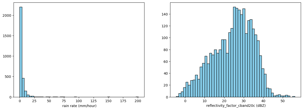

This looks as expected. There are some higher values of rain rates.

fig, axes = plt.subplots(2, 1, figsize=(12, 8), sharex=True) 

ds['rain_rate'].plot(ax=axes[0], color='blue')
axes[0].set_title('Time Series of rain_rate')
axes[0].set_ylabel(f'{ds["rain_rate"].long_name} ({ds["rain_rate"].units})')

ds['reflectivity_factor_cband20c'].plot(ax=axes[1], color='blue')
axes[1].set_title('Time Series of reflectivity_factor_cband20c')
axes[1].set_ylabel(f'{ds["reflectivity_factor_cband20c"].long_name} ({ds["reflectivity_factor_cband20c"].units})')

plt.xlabel('Time')
plt.tight_layout()
plt.show()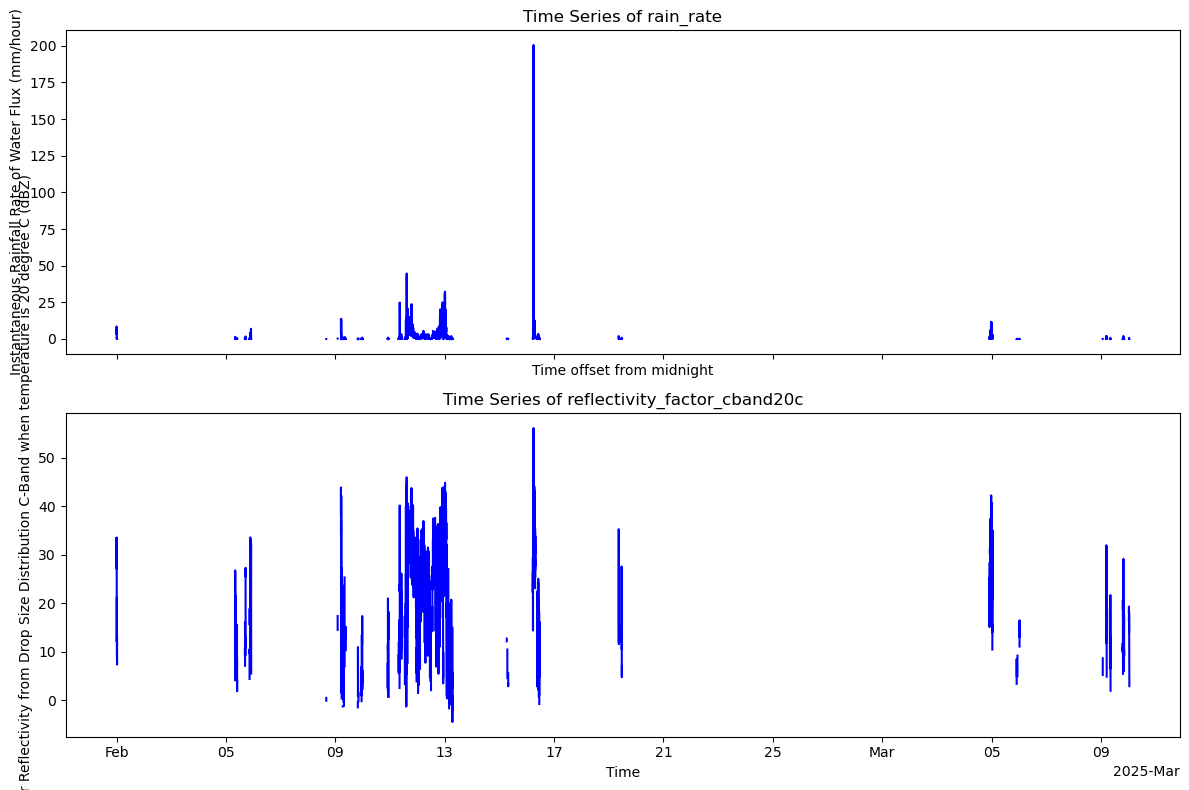

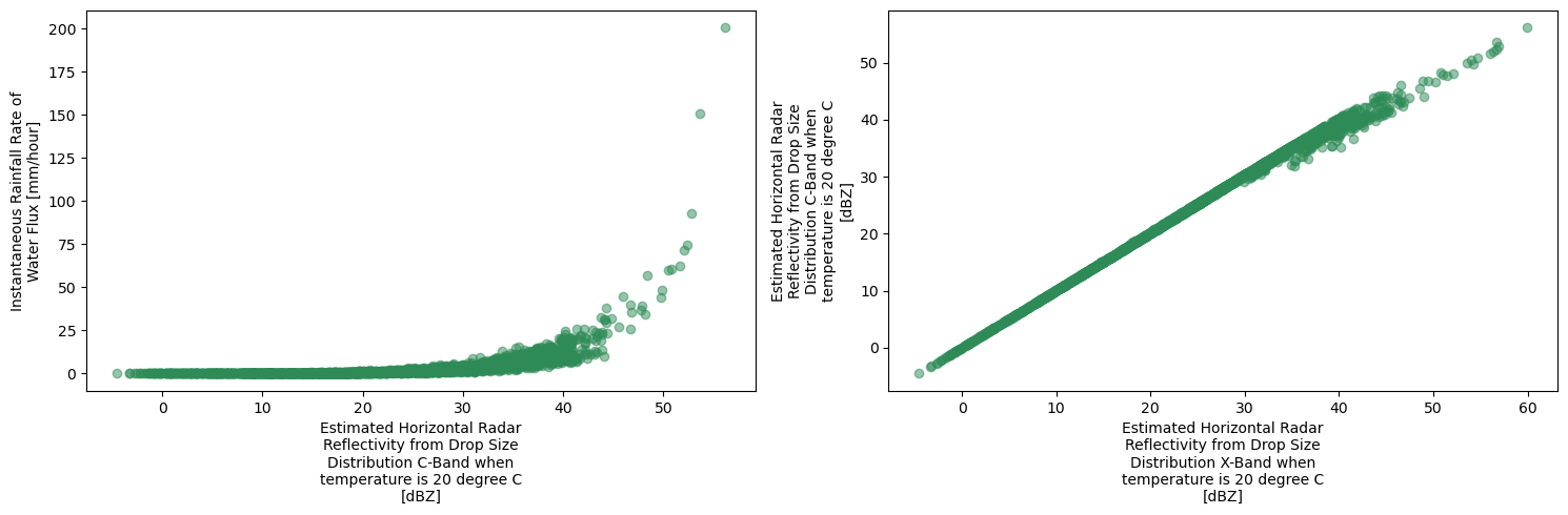
Some more plots. ZR plot is looking promising.

fig, axes = plt.subplots(1, 2, figsize=(15, 5))

ds.plot.scatter(x='reflectivity_factor_cband20c', y='rain_rate', ax=axes[0], alpha=0.5, color='seagreen')
ds.plot.scatter(x='reflectivity_factor_xband20c', y='reflectivity_factor_cband20c', ax=axes[1], alpha=0.5, color='seagreen')

plt.tight_layout()
plt.show()

Fitting ZR relationship¶

To find the coefficients a and b in the power-law relationship Z = a * R^b, we do linear regression in log-log space. Take Log of both sides of the Z-R equation gives

log(Z) = log(a) + b * log(R)

# let me first remove bad values, as i think that is causing issues
rain_rate = ds['rain_rate'].values 
reflectivity_dbz = ds['reflectivity_factor_cband20c'].values

valid_indices_zr = np.where(np.isfinite(rain_rate) & np.isfinite(reflectivity_dbz) & (rain_rate > 0)) # remove bad values
rain_rate = rain_rate[valid_indices_zr]
reflectivity_dbz = reflectivity_dbz[valid_indices_zr]

print(f"Min dBZ: {min(reflectivity_dbz)}")
print(f"Max dBZ: {max(reflectivity_dbz)}")

Min dBZ: -4.522533893585205
Max dBZ: 56.1351432800293

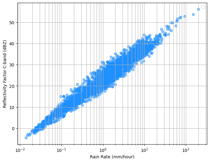
Plot Log-Log relationship¶

plt.figure(figsize=(8, 6))
plt.scatter(rain_rate, reflectivity_dbz, alpha=0.5, color='dodgerblue')
plt.xlabel('Rain Rate (mm/hour)')
plt.ylabel('Reflectivity Factor C-band (dBZ)')
plt.xscale('log') # Logarithmic scale for rain rate
plt.yscale('linear')
plt.grid(True, which="both", ls="-")
plt.legend()
plt.show()

No artists with labels found to put in legend.  Note that artists whose label start with an underscore are ignored when legend() is called with no argument.

Z_linear = 10**(reflectivity_dbz / 10) # Z in mm^6 m^-3
log_Z = np.log10(Z_linear) # Take log10 of Z
log_R = np.log10(rain_rate) # Take log10 of rain rate
plt.plot(log_R, log_Z, 'o', color='blue', alpha=0.5)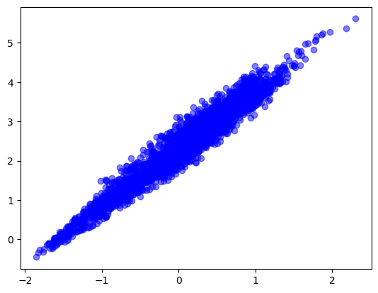

Linear regression¶

coefficients_zr = np.polyfit(log_R, log_Z, 1) # Linear fit: log(Z) = b*log(R) + log(a)
print(f"coefficients_zr (raw from np.polyfit): {coefficients_zr}")
b_coefficient = coefficients_zr[0] # Slope
log_a_coefficient = coefficients_zr[1] # Intercept
a_coefficient = 10**log_a_coefficient # Convert to a

print(f"Z-R Relationship for C-band (from LDQUANTS data):")
print(f"Z = {a_coefficient:.2f} * R**{b_coefficient:.2f}") # Z = a * R^b

coefficients_zr (raw from np.polyfit): [1.46141458 2.33188229]
Z-R Relationship for C-band (from LDQUANTS data):
Z = 214.72 * R**1.46

plt.figure(figsize=(8, 6))
plt.scatter(rain_rate, reflectivity_dbz, alpha=0.5, color='dodgerblue')
plt.xlabel('Rain Rate (mm/hour)')
plt.ylabel('Reflectivity Factor C-band (dBZ)')
plt.xscale('log') # Logarithmic scale for rain rate
plt.yscale('linear')
plt.grid(True, which="both", ls="-")

# Add the fitted Z-R line
rain_rate_line = np.logspace(np.log10(min(rain_rate)), np.log10(max(rain_rate)), 100)
Z_linear_line = a_coefficient * (rain_rate_line**b_coefficient)
reflectivity_dbz_line = 10 * np.log10(Z_linear_line)
plt.plot(rain_rate_line, reflectivity_dbz_line, color='blue', linewidth=2, label=f'Fitted Z-R: Z={a_coefficient:.2f}*R**{b_coefficient:.2f}')

plt.legend()
plt.show()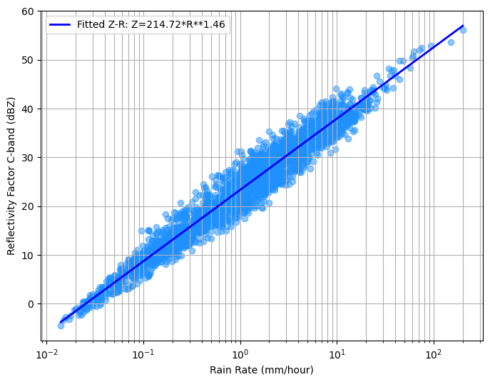

Now this is correct!

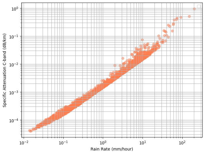
Now we will do the same for Attenuation¶

rain_rate = ds['rain_rate'].values 
specific_attenuation = ds['specific_attenuation_cband20c'].values

valid_indices_kr = np.where(np.isfinite(rain_rate) & np.isfinite(specific_attenuation) & (rain_rate > 0)) # remove bad values or it will cause iisues
rain_rate = rain_rate[valid_indices_kr] 
specific_attenuation = specific_attenuation[valid_indices_kr]

print(f"Min specific_attenuation (dB/km): {min(specific_attenuation)}")
print(f"Max specific_attenuation (dB/km): {max(specific_attenuation)}")

Min specific_attenuation (dB/km): 3.992306665168144e-05
Max specific_attenuation (dB/km): 0.9515843391418457

plt.figure(figsize=(8, 6))
plt.scatter(rain_rate, specific_attenuation, alpha=0.5, color='coral') 
plt.xlabel('Rain Rate (mm/hour)')
plt.ylabel('Specific Attenuation C-band (dB/km)')
plt.xscale('log')
plt.yscale('log')
plt.grid(True, which="both", ls="-")
plt.legend()
plt.show()

No artists with labels found to put in legend.  Note that artists whose label start with an underscore are ignored when legend() is called with no argument.

log_R_k = np.log10(rain_rate) 
log_k = np.log10(specific_attenuation)

coefficients_kr = np.polyfit(log_R_k, log_k, 1) # Linear fit: log(k) =d*log(R) + log(c)
print(f"coefficients_kr (raw from np.polyfit): {coefficients_kr}")
d_coefficient = coefficients_kr[0] # Slope is d
log_c_coefficient = coefficients_kr[1] # Intercept
c_coefficient = 10**log_c_coefficient # Convert to c

print(f"k-R Relationship for C-band (from LDQUANTS data)")
print(f"k = {c_coefficient:.3f} * R**{d_coefficient:.3f}") # k= c * R**d

coefficients_kr (raw from np.polyfit): [ 0.99072717 -2.76246926]
k-R Relationship for C-band (from LDQUANTS data)
k = 0.002 * R**0.991

Let’s check it.

plt.figure(figsize=(8, 6))
plt.scatter(rain_rate, specific_attenuation, alpha=0.5, color='coral') 

rain_rate_fit_kr = np.linspace(min(rain_rate), max(rain_rate), 100) 
attenuation_fit = c_coefficient * (rain_rate_fit_kr**d_coefficient) 

plt.plot(rain_rate_fit_kr, attenuation_fit, color='red', 
         linewidth=2, label=f'Fitted k-R: k={c_coefficient:.3f}*R**{d_coefficient:.3f}')

plt.ylabel('Specific Attenuation C-band (dB/km)')
plt.title('k-R Relationship derived from LDQUANTS (C-band) data')
plt.xscale('log') 
plt.yscale('log') 
plt.grid(True, which="both", ls="-")
plt.legend()
plt.xlim(min(rain_rate)*0.8, max(rain_rate)*1.2) 
plt.ylim(min(specific_attenuation)*0.8, max(specific_attenuation)*1.2)
plt.show()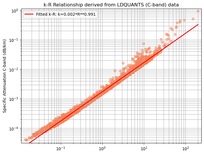

Because the one rain event was mainly convective the attenuation relationship was looking better, however it has issues with higher rain rates.

Site Exploration

Bankhead National Forest In-Situ Observation Locations

Extracted Radar Columns and In-Situ Sensors

Bankhead National Forest - RadClss Example