Bankhead National Forest In-Situ Observation Locations
Overview
For the Extracted Radar Columns and In-Situ Sensors (RadCLss) Product, investigation of the location of available in-situ sensors with respect to the C-SAPR2 is desired.
This notebook utilizes GeoPandas and Cartopy to map various observational assets around the ARM AMF site and creates displays of:
ARM Mobile Facility (AMF) Main Site.
3rd Party Observational Networks.
Spatial Display for Potential RadCLss columns.
Prerequisites
| Concepts | Importance | Notes |
|---|---|---|
| Intro to Cartopy | Necessary | |
| Understanding of NetCDF | Helpful | Familiarity with metadata structure |
| GeoPandas | Necessary |
Time to learn: estimate in minutes. For a rough idea, use 5 mins per subsection, 10 if longer; add these up for a total. Safer to round up and overestimate.
System requirements:
Populate with any system, version, or non-Python software requirements if necessary
Otherwise use the concepts table above and the Imports section below to describe required packages as necessary
If no extra requirements, remove the System requirements point altogether
Imports
import fiona
import warnings

import matplotlib.pyplot as plt
import geopandas as gpd
from metpy.plots import USCOUNTIES

from cartopy import crs as ccrs, feature as cfeature
from cartopy.io.img_tiles import OSM

fiona.drvsupport.supported_drivers['libkml'] = 'rw' # enable KML support which is disabled by default
fiona.drvsupport.supported_drivers['LIBKML'] = 'rw' # enable KML support which is disabled by default

warnings.filterwarnings("ignore", category=RuntimeWarning)
warnings.filterwarnings("ignore", category=UserWarning)
ARM Mobile Facility (AMF) Main Site
Read in the KMZ file provide by the ARM site operations team
# note: the KMZ file provided contains multiple geometry columns.
in_layers = []
for layer in fiona.listlayers("locations/BNF.kmz"):
    print(layer)
    s = gpd.read_file("locations/BNF.kmz", layer=layer)
    in_layers.append(s)
BNF_Schematic
M1
S10
S13
S14
S20
S30
S40
S3
S4
Original_Proclaimed_National_Forests_and_National_Grasslands_(Feature_Layer).kml
Original_Proclaimed_National_Forests_and_National_Grasslands__Feature_Layer_
Inspect the GeoPandas DataFrames
# Overall BNF Schematic
in_layers[0]# Display all the layers
in_layers[0].plot()<Axes: >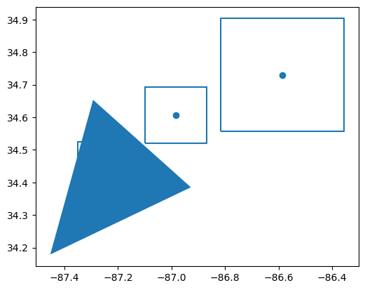
# Display the `BNF Airshed`
in_layers[0].loc[[1], 'geometry'].plot()
<Axes: >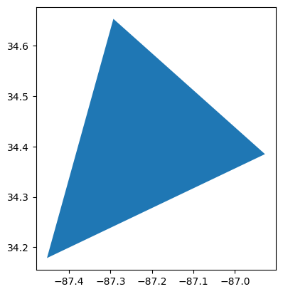
# Inspect the ARM AMF M1 GeoDataFrame
in_layers[1]in_layers[1].iloc[4]Name M1
description NaN
timestamp NaT
begin NaT
end NaT
altitudeMode NaN
tessellate -1
extrude 0
visibility -1
drawOrder NaN
icon NaN
geometry POINT Z (-87.33841564329165 34.34525430686622 0)
Name: 4, dtype: object# BNF Forest Outline
in_layers[11].plot(facecolor="None", edgecolor="black")<Axes: >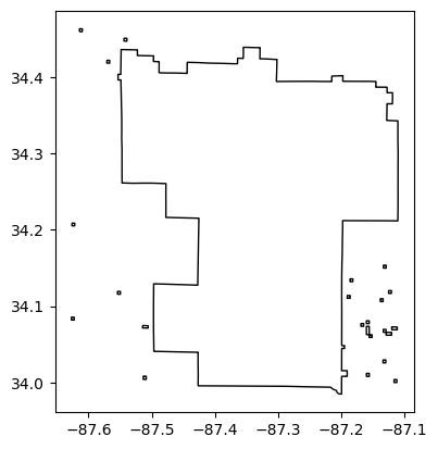
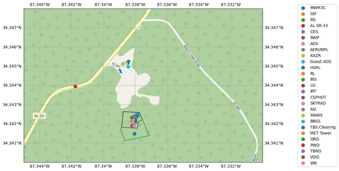
ARM AMF M1 Site Display
# Set up the figure
fig = plt.figure(figsize=(14, 7))
# Initialize OpenStreetMap tile
tiler = OSM()
# Create a subplot and define projection
ax = fig.add_subplot(1, 1, 1, projection=ccrs.PlateCarree())

# Add some various map elements to the plot to make it recognizable.
# Initialize OpenStreetMap tile
tiler = OSM()
ax.add_feature(cfeature.COASTLINE)
ax.add_feature(cfeature.STATES)
ax.add_feature(cfeature.BORDERS)
ax.add_image(tiler, 16, zorder=1)
# Set the BNF Domain (adjust later for various groups)
ax.set_extent([272.655, 272.67, 34.340, 34.348])
ax.gridlines(draw_labels=True)

for index in in_layers[1].index:
    # Skipping fence marking and main instrument field polygons, leaving instruments
    # Was making legend messy, and unable to set right side gridlines to false
    if index != 5 and index != 29:
        if in_layers[1].loc[[index], 'Name'].values[0] == "TBS Planned Clearing":
                in_layers[1].loc[[index], 'geometry'].plot(transform=ccrs.PlateCarree(),
                                                           ax=ax,
                                                           label=in_layers[1].loc[[index], 'Name'].values[0],
                                                           zorder=2,
                                                           facecolor="none",
                                                           edgecolor="green",
                                                           markersize=65)
        elif in_layers[1].loc[[index], 'Name'].values[0] == "Main Instrument Field Already Cleared":
                in_layers[1].loc[[index], 'geometry'].plot(transform=ccrs.PlateCarree(),
                                                           ax=ax,
                                                           label=in_layers[1].loc[[index], 'Name'].values[0],
                                                           zorder=2,
                                                           facecolor="none",
                                                           markersize=65)
        else:
            in_layers[1].loc[[index], 'geometry'].plot(transform=ccrs.PlateCarree(),
                                                       ax=ax,
                                                       label=in_layers[1].loc[[index], 'Name'].values[0],
                                                       zorder=2,
                                                       markersize=65)

ax.spines['right'].set_visible(False)
# Add a legend
# Place a legend to the right of this smaller subplot.
fig.legend(loc='right')

# Set the DPI to a higher value (e.g., 300)
plt.rcParams['figure.dpi'] = 300
plt.rcParams['savefig.dpi'] = 300
3rd Party Observational Network
site_locations = gpd.read_file("locations/ARM-SE.kmz")
site_locations# Set up the figure
fig = plt.figure(figsize=(14, 7))
# Initialize OpenStreetMap tile
tiler = OSM()
# Create a subplot and define projection
ax = fig.add_subplot(1, 1, 1, projection=ccrs.PlateCarree())
# Add some various map elements to the plot to make it recognizable.
# Initialize OpenStreetMap tile
tiler = OSM()
ax.add_feature(cfeature.COASTLINE)
ax.add_feature(cfeature.STATES)
ax.add_feature(cfeature.BORDERS)
ax.add_image(tiler, 7, zorder=1)
# Set the BNF Domain (adjust later for various groups)
ax.set_extent([270.0, 276.0, 36.0, 30.0])
ax.gridlines(draw_labels=True)
for index in site_locations.index:
site_locations.loc[[index], 'geometry'].plot(transform=ccrs.PlateCarree(),
ax=ax,
label=site_locations.loc[[index], 'Name'].values[0],
zorder=2,
markersize=65)
# Add a legend
# Place a legend to the right of this smaller subplot.
fig.legend(loc='right')
# Set the DPI to a higher value (e.g., 300)
plt.rcParams['figure.dpi'] = 300
plt.rcParams['savefig.dpi'] = 300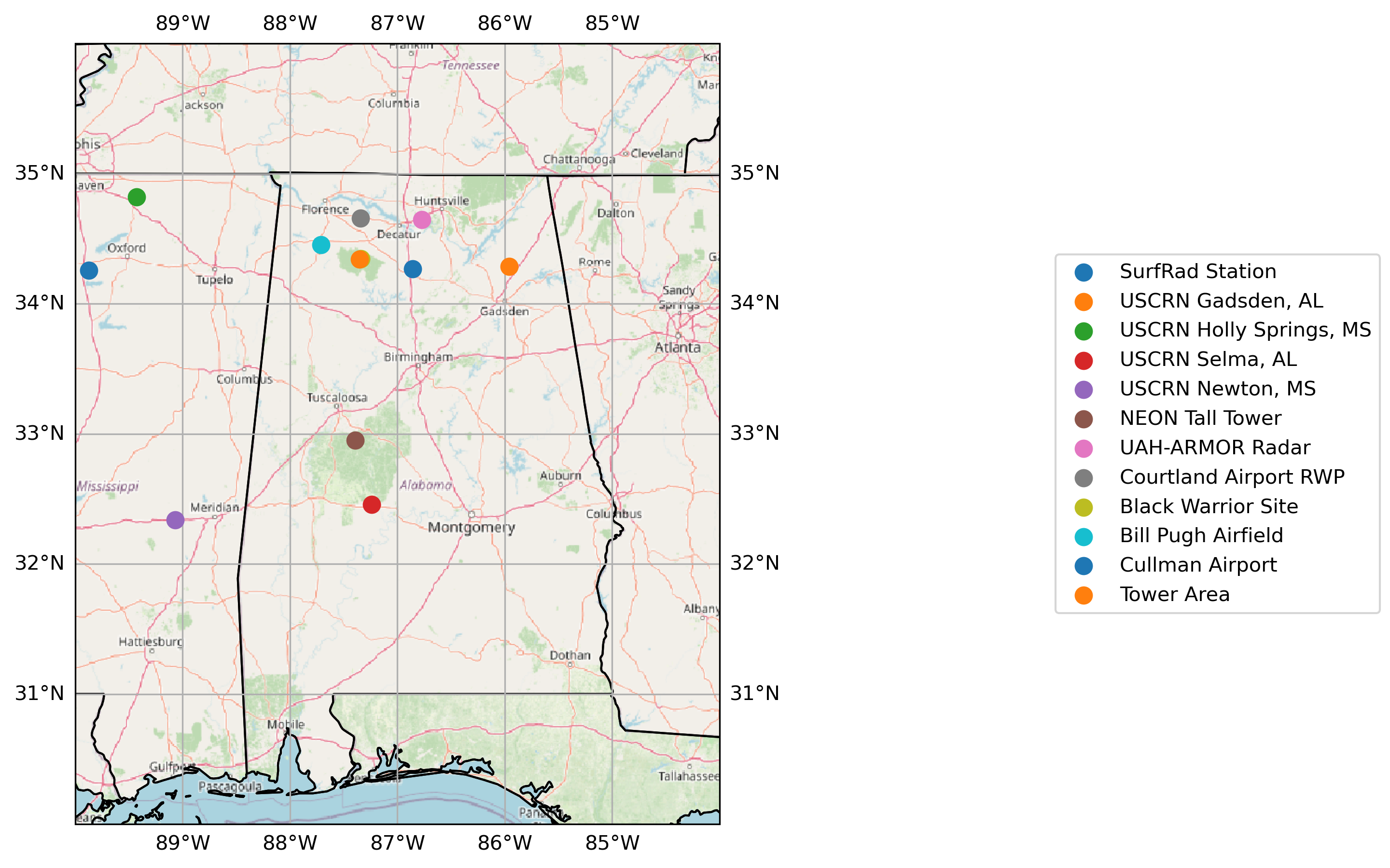
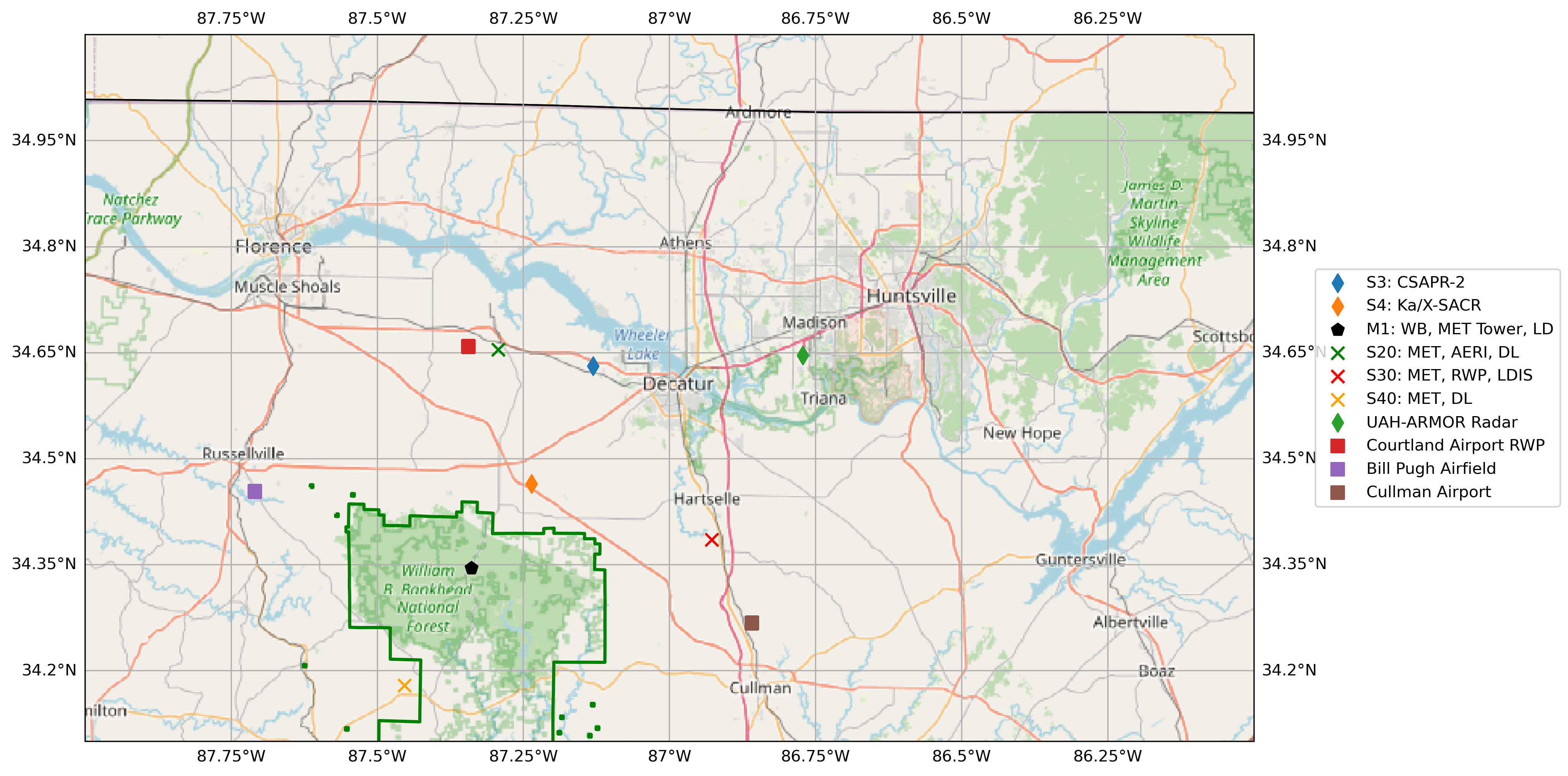
Spatial Display for Potential RadCLss Columns
# define the center of the map to be the CSAPR2
central_lon = -87.13076
central_lat = 34.63080

# Set up the figure
fig = plt.figure(figsize=(16, 8))
# Initialize OpenStreetMap tile
tiler = OSM()
# Create a subplot and define projection
ax = fig.add_subplot(1, 1, 1, projection=ccrs.PlateCarree())

# Add some various map elements to the plot to make it recognizable.
# Initialize OpenStreetMap tile
tiler = OSM()
ax.add_feature(cfeature.COASTLINE)
ax.add_feature(cfeature.STATES)
ax.add_feature(cfeature.BORDERS)
ax.add_image(tiler, 9, zorder=1)
# Set the BNF Domain (adjust later for various groups)
ax.set_extent([272.0, 274.0, 35.1, 34.1])
ax.gridlines(draw_labels=True)

# add in kmz file layers
# BNF Forest Preserve Land
in_layers[11].plot(transform=ccrs.PlateCarree(),
                   facecolor="none",
                   edgecolor="green",
                   linewidth=2.0,
                   ax=ax,
                   label="BNF Forest Preserve",
                   zorder=2)
# CSAPR2 location
in_layers[8].plot(transform=ccrs.PlateCarree(),
                  ax=ax,
                  label="S3: CSAPR-2",
                  zorder=2,
                  marker="d",
                  markersize=65)
# X-SAPR location
in_layers[9].plot(transform=ccrs.PlateCarree(),
                  ax=ax,
                  label="S4: Ka/X-SACR",
                  zorder=2,
                  marker="d",
                  markersize=65)
# M1 location
in_layers[1].loc[[4], 'geometry'].plot(transform=ccrs.PlateCarree(),
                                       ax=ax,
                                       label="M1: WB, MET Tower, LD",
                                       zorder=2,
                                       marker="p",
                                       color="black",
                                       markersize=65)

# S20 location - MET, AERI, DL
in_layers[5].plot(transform=ccrs.PlateCarree(),
                          ax=ax,
                          label="S20: MET, AERI, DL",
                          zorder=2,
                          marker="x",
                          color="green",
                          markersize=65)

# S30 location - MET, RWP, LDIS
in_layers[6].plot(transform=ccrs.PlateCarree(),
                          ax=ax,
                          label="S30: MET, RWP, LDIS",
                          zorder=2,
                          marker="x",
                          color="red",
                          markersize=65)

# S40 location - MET, AERI, DL
in_layers[7].plot(transform=ccrs.PlateCarree(),
                          ax=ax,
                          label="S40: MET, DL",
                          zorder=2,
                          marker="x",
                          color="orange",
                          markersize=65)

# Add in the 3rd Party Sites
site_locations.loc[[6], 'geometry'].plot(transform=ccrs.PlateCarree(),
                                         ax=ax,
                                         label=site_locations.loc[[6], 'Name'].values[0],
                                         zorder=2,
                                         markersize=65,
                                         marker='d')
site_locations.loc[[7], 'geometry'].plot(transform=ccrs.PlateCarree(),
                                         ax=ax,
                                         label=site_locations.loc[[7], 'Name'].values[0],
                                         zorder=2,
                                         markersize=65,
                                         marker='s')
site_locations.loc[[9], 'geometry'].plot(transform=ccrs.PlateCarree(),
                                         ax=ax,
                                         label=site_locations.loc[[9], 'Name'].values[0],
                                         zorder=2,
                                         markersize=65,
                                         marker='s')
site_locations.loc[[10], 'geometry'].plot(transform=ccrs.PlateCarree(),
                                         ax=ax,
                                         label=site_locations.loc[[10], 'Name'].values[0],
                                         zorder=2,
                                         markersize=65,
                                         marker='s')

# Add a legend
# Place a legend to the right of this smaller subplot.
fig.legend(loc='right')

# Set the DPI to a higher value (e.g., 300)
plt.rcParams['figure.dpi'] = 300
plt.rcParams['savefig.dpi'] = 300