Bankhead National Forest - RadCLss Met Tower
Overview
The Extracted Radar Columns and In-Situ Sensors (RadClss) Value-Added Product (VAP) is a dataset containing in-situ ground observations matched to CSAPR-2 radar columns above ARM Mobile Facility (AMF-3) supplemental sites of interest.
Investigation into specific azimuth and range gate separation over the BNF Met Tower Site to see if RadCLss can differeniate between these close locations
Prerequisites
| Concepts | Importance | Notes |
|---|---|---|
| Intro to Cartopy | Necessary | |
| Understanding of NetCDF | Helpful | Familiarity with metadata structure |
| GeoPandas | Necessary | Familiarity with Geospatial Plotting |
| Py-ART / Radar Foundations | Necessary | Basics of Weather Radar |
Time to learn: 30 minutes
In-Situ Locations
| Site | Lat | Lon | Forward Azimuth | Distance |
|---|---|---|---|---|
| M1 | 34.34525 | -87.33842 | 210.709 | 36.909 |
| S4 | 34.46451 | -87.23598 | 207.027 | 20.753 |
| S20 | 34.65401 | -87.29264 | 280.072 | 14.82 |
| S30 | 34.38501 | -86.92757 | 145.371 | 33.192 |
| S40 | 34.17932 | -87.45349 | 210.438 | 58.174 |
| S10. | 34.34361 | -87.35027 | 211.995 | 37.629 |
| S13. | 34.34388 | -87.35055 | 212.053 | 37.616 |
| S14. | 34.34333 | -87.35083 | 212.036 | 37.682 |
import warnings
warnings.filterwarnings("ignore", category=DeprecationWarning)

import glob
import os
import datetime
import tempfile
from datetime import timedelta

import numpy as np
import matplotlib.pyplot as plt
import matplotlib.gridspec as gridspec
import xarray as xr
import pandas as pd
import dask
import cartopy
import cartopy.crs as ccrs

from math import atan2 as atan2
from cartopy import crs as ccrs, feature as cfeature
from cartopy.io.img_tiles import OSM
from matplotlib.transforms import offset_copy
from mpl_toolkits.axes_grid1 import make_axes_locatable
from mpl_toolkits.axisartist.grid_finder import FixedLocator, DictFormatter
from matplotlib import colors
from dask.distributed import Client, LocalCluster
from metpy.plots import USCOUNTIES
from PIL import Image

import act
import pyart
import wradlib as wrl
import cmweather
import xradar as xd

dask.config.set({'logging.distributed': 'error'})
<dask.config.set at 0x328f48e50>Read CSAPR-2 Data with xradar and visualize with wradlib
# Define the desired processing date for the BNF CSAPR-2 in YYYY-MM-DD format.
DATE = "2025-03-05"
# Define the directory where the BNF CSAPR-2 CMAC files are located.
RADAR_DIR = sorted(glob.glob(os.getenv("BNF_RADAR_R5_DIR") + "202503/*.nc"))
dt = xd.io.open_cfradial1_datatree(RADAR_DIR[-2])dtLoading...
dt['sweep_0']['corrected_reflectivity']Loading...
dt['sweep_0']['corrected_reflectivity'].plot()
Extract the lowest sweep
ds = dt['sweep_0'].to_dataset()dsLoading...
wradlib visualization
da = ds['corrected_reflectivity']# note - required metadata for wradlib visualization / georeferencing
da.attrs['sweep_mode'] = 'azimuth_surveillance'da = da.wrl.georef.georeference()daLoading...
da.wrl.vis.plot()
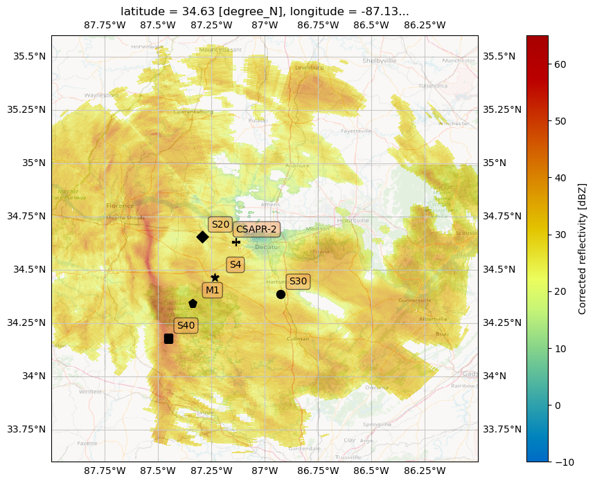
Overaly the OpenStreetMap on wradlib visualization
# define the sites of interest
nsite = {"M1" : [34.34525, -87.33842],
         "S4" : [34.46451, -87.23598],
         "S3" : [34.63080, -87.13311],
         "S20" : [34.65401, -87.29264],
         "S30" : [34.38501, -86.92757],
         "S40" : [34.17932, -87.45349],
         "S10" : [34.34361, -87.35027],
         "S13" : [34.34388, -87.35055],
         "S14" : [34.34333, -87.35083]}

# define the center of the map to be the CSAPR2
central_lon = -87.13076
central_lat = 34.63080
fig = plt.figure(figsize=(18, 8))
tiler = OSM()
mercator = tiler.crs
ax = fig.add_subplot(111,
projection=ccrs.PlateCarree())
# Add some various map elements to the plot to make it recognizable.
ax.add_feature(cfeature.COASTLINE)
ax.add_image(tiler, 9, zorder=2, alpha=0.4)
# Set the BNF Domain (adjust later for various groups)
ax.set_extent([272.0, 274.0, 35.1, 34.1])
gl = ax.gridlines(draw_labels=True)
# Hide the right side ticks
ax.tick_params(labeltop=False, labelright=False)
# Add the column sites
markers = ["p", "*", "+", "D", "o", "s"]
for i, site in enumerate(nsite):
ax.scatter(nsite[site][1],
nsite[site][0],
marker=markers[i],
color="black",
s=75,
label=site,
zorder=3,
transform=ccrs.PlateCarree())
# Use the cartopy interface to create a matplotlib transform object
# for the Geodetic coordinate system. We will use this along with
# matplotlib's offset_copy function to define a coordinate system which
# translates the text by 25 pixels to the left.
# note - taken from cartopy examples
geodetic_transform = ccrs.PlateCarree()._as_mpl_transform(ax)
text_transform = offset_copy(geodetic_transform, units='dots', x=+50, y=+15)
if site == "S3":
# Add text upper right of the site marker.
ax.text(nsite[site][1]+0.03,
nsite[site][0]+0.01,
"CSAPR-2",
verticalalignment='center',
horizontalalignment='right',
transform=text_transform,
bbox=dict(facecolor='sandybrown',
alpha=0.5,
boxstyle='round'))
else:
# Add text upper right of the site marker.
ax.text(nsite[site][1]-0.035,
nsite[site][0]+0.01,
site,
verticalalignment='center',
horizontalalignment='right',
transform=text_transform,
bbox=dict(facecolor='sandybrown',
alpha=0.5,
boxstyle='round'))
cg = {"radial_spacing": 10.0, "latmin": 34}
da.wrl.vis.plot(ax=ax,
vmin=-10,
vmax=65)<cartopy.mpl.geocollection.GeoQuadMesh at 0x30d7731d0>Ignoring fixed y limits to fulfill fixed data aspect with adjustable data limits.
Sector Curvelinear Grid - PPI - Bankhead National Forest
# very basic curvelinear graph
fig = plt.figure(figsize=(8, 8))
pm = da.wrl.vis.plot(fig=fig, crs='cg')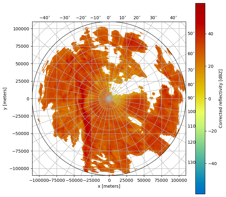
cg = {"angular_spacing": 5.0}
fig = plt.figure(figsize=(10, 8))
sel = da.sel(azimuth=slice(200, 225), range=slice(20000, 60000))
pm = sel.wrl.vis.plot(
    fig=fig,
    crs=cg,
    infer_intervals=True,
)
cgax = plt.gca() # main axis
caax = cgax.parasites[0] # cartesian axis
paax = cgax.parasites[1] # polar axis

t = plt.title("CSAPR-2 Sector CG PPI", y=1.05)
cbar = plt.gcf().colorbar(pm, pad=0.075, ax=cgax)
caax.set_xlabel("x_range [m]")
caax.set_ylabel("y_range [m]")
plt.text(1.0, 1.05, "azimuth", transform=caax.transAxes, va="bottom", ha="right")

# set azimuth resolution to 5deg and display
gh = cgax.get_grid_helper()
locs = [i for i in np.arange(0.0, 360.0, 5)]
gh.grid_finder.grid_locator1 = FixedLocator(locs)
gh.grid_finder.tick_formatter1 = DictFormatter(
    dict([(i, r"${0:.0f}^\circ$".format(i)) for i in locs])
)
# Define the number of range ticks
gh.grid_finder.grid_locator2._nbins = 10
#gh.grid_finder.grid_locator2._steps = [1, 1.5, 2, 2.5, 5, 10]
cgax.axis["lat"] = cgax.new_floating_axis(0, 225)
cgax.axis["lat"].set_ticklabel_direction("-")
cgax.axis["lat"].label.set_text("range [m]")
cgax.axis["lat"].label.set_rotation(180)
cgax.axis["lat"].label.set_pad(10)

# Plot sites on the polar Axis
paax.plot(210.709, 36909, "bo", label="M1", zorder=1)
paax.plot(207.027, 20753, "ro", label="S4", zorder=1)
paax.plot(210.438, 58174, "go", label="S40", zorder=1)

handles, labels = cgax.get_legend_handles_labels()
by_label = dict(zip(labels, handles))
cgax.legend(by_label.values(),
            by_label.keys(),
            loc="upper left",    # whatever placement you want
            title="Site ID")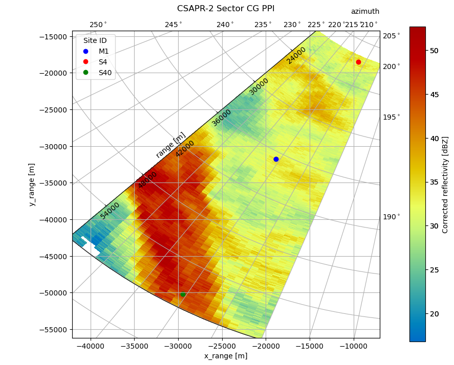
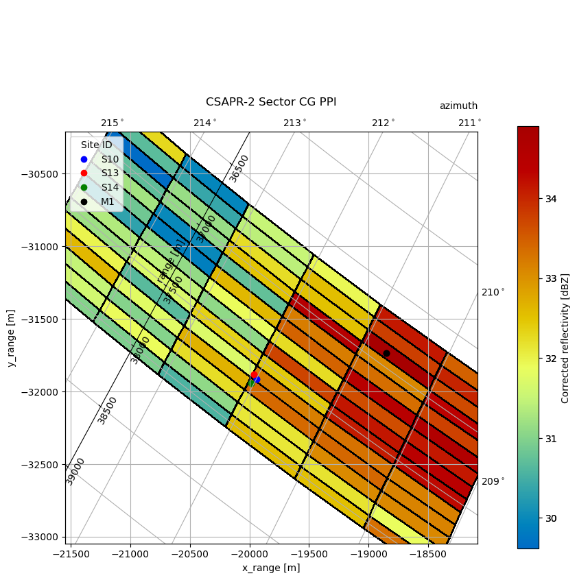
CV Grid over BNF Tall Tower Site
cg = {"angular_spacing": 5.0}
fig = plt.figure(figsize=(10, 8))
sel = da.sel(azimuth=slice(209, 215), range=slice(36680, 38000))
pm = sel.wrl.vis.plot(
    fig=fig,
    crs=cg,
    infer_intervals=True,
    edgecolors='black'
)
cgax = plt.gca() # main axis
caax = cgax.parasites[0] # cartesian axis
paax = cgax.parasites[1] # polar axis

t = plt.title("CSAPR-2 Sector CG PPI", y=1.05)
cbar = plt.gcf().colorbar(pm, pad=0.075, ax=cgax)
caax.set_xlabel("x_range [m]")
caax.set_ylabel("y_range [m]")
plt.text(1.0, 1.05, "azimuth", transform=caax.transAxes, va="bottom", ha="right")

# set azimuth resolution to 5deg and display
gh = cgax.get_grid_helper()
locs = [i for i in np.arange(0.0, 360.0, 1)]
gh.grid_finder.grid_locator1 = FixedLocator(locs)
gh.grid_finder.tick_formatter1 = DictFormatter(
    dict([(i, r"${0:.0f}^\circ$".format(i)) for i in locs])
)
# Define the number of range ticks
gh.grid_finder.grid_locator2._nbins = 10
#gh.grid_finder.grid_locator2._steps = [1, 1.5, 2, 2.5, 5, 10]
cgax.axis["lat"] = cgax.new_floating_axis(0, 213.5)
cgax.axis["lat"].set_ticklabel_direction("-")
cgax.axis["lat"].label.set_text("range [m]")
cgax.axis["lat"].label.set_rotation(180)
cgax.axis["lat"].label.set_pad(10)

# Plot sites on the polar Axis
paax.plot(211.995, 37629, "bo", label="S10", zorder=1)
paax.plot(212.053, 37616, "ro", label="S13", zorder=1)
paax.plot(212.036, 37682, "go", label="S14", zorder=1)
paax.plot(210.709, 36909, "ko", label="M1", zorder=1)

handles, labels = cgax.get_legend_handles_labels()
by_label = dict(zip(labels, handles))
cgax.legend(by_label.values(),
            by_label.keys(),
            loc="upper left",    # whatever placement you want
            title="Site ID")