Decadal Near-Surface Turbulent Flux Measurements from ARM¶

Overview¶

Within this notebook, we will cover the methodology and analysis within Sullivan et al. (2025) :

History of near 3 decades of ARM’s near-surface turbulent flux observations
Introduction to the Energy Balance Bowen Ratio (EBBR) and Eddy Covariance (EC) methods
Comparison of Sensible and Latent Heat Fluxes from these methods for 2015 to 2023 period at SGP

Prerequisites¶

Concepts	Importance	Notes
ACT Basics	Helpful	Basic features
Matplotlib Basics	Helpful	Basic plotting
NumPy Basics	Helpful	Basic arrays
Xarray Basics	Helpful	Multi-dimensional arrays

Time to learn: 15 minutes

History of ARM’s Near-Surface Turbulent Flux Observations at SGP¶

Sensible and latent heat fluxes (H and LE) are critical to modulating the sources and sinks of the energy and water budgets across the land-atmosphere-biosphere interface.

In-situ measurements of H and LE are critical for understanding and predicting processes relevant for heat waves, droughts, argiculture and irrigation scheduling, and are necessary to capture the fine scale scales at which these processes occur.

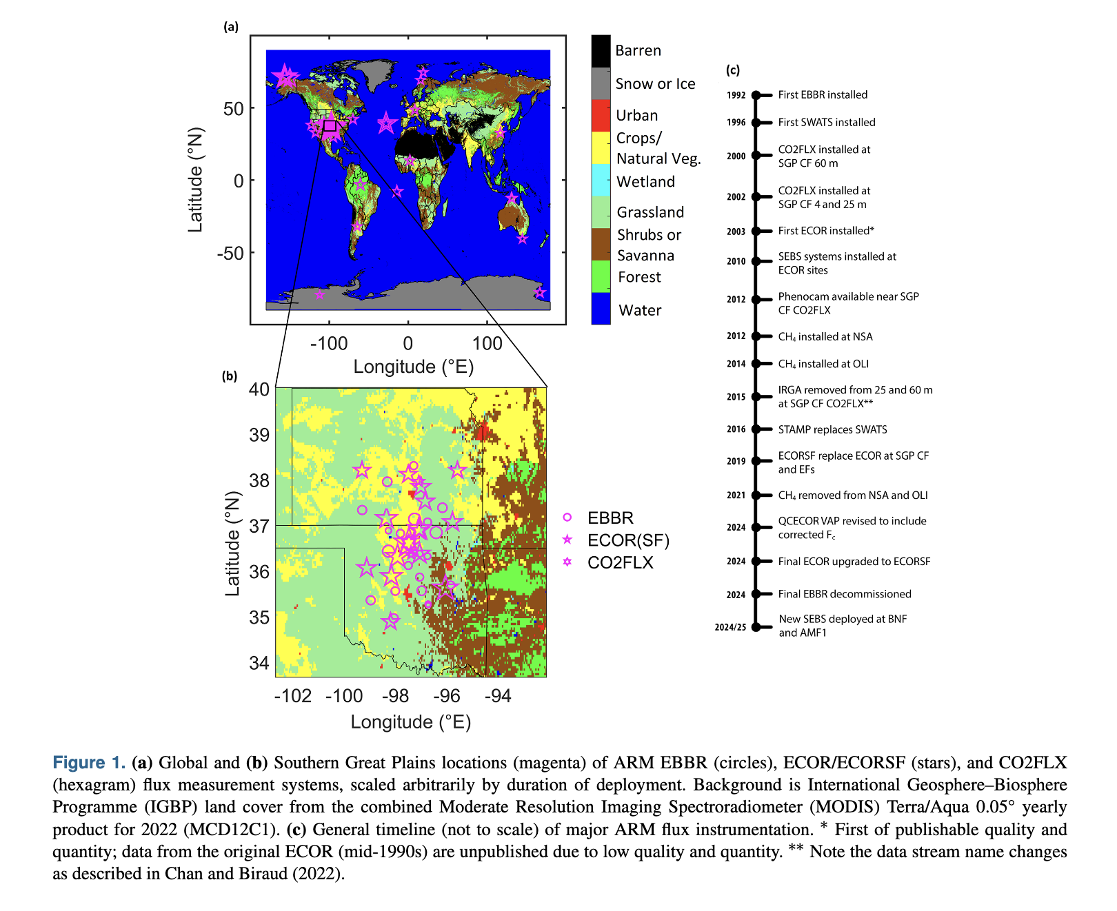
The U.S. Department of Energy (DOE) Atmospheric Radiation Measurement (ARM) user facility has measured fluxes primarily using in-situ meteorologically driven energy balance flux gradient method with energy balance Bowen ratio (EBBR) system, the eddy covariance method (EC) with the carbon dioxide flux (CO2FLX), and the eddy correlation (ECOR) flux measurement system.

ARM began measuring fluxes in 1992 ^[1] using the EBBR system at the Southern Great Plains (SGP) atmospheric observatory, at ten grassland extended facilities (EF) within Oklahoma and Kansas and one EF on the northern edge of cropland. THe intention was that these facilities would be representative of a typical global climate model (GCM) grid cell.

The Energy Balence Bowen Ratio (EBBR) Method¶

The EBBR measures near-surface gradients of temperature and humidty^[2] to approximate the Bowen Ratio:

\beta \equiv \frac{H}{LE} \approx \frac{C_p \rho}{\lambda}\frac{\overline{\Delta T}}{\overline{\Delta \rho_v}},

(1)

where:

$\beta$ is the Bowen ratio
$H$ is the sensible heat flux
$LE$ is the latent heat flux
$C_p$ is the specific heat of air ( $\mathrm{J\ kg^{-1}\ K^{-1}}$ )
$\rho$ is the density of air ( $\mathrm{kg\ m^{-3}}$ )
$\lambda$ is the latent heat of vaporization of water (or the latent heat of sublimation for frozen conditions) ( $\mathrm{J\ kg^{-1}}$ )
$\overline{\Delta T}$ is the mean temperature difference between the upper and lower sensors ( $\mathrm{K}$ )
$\overline{\Delta \rho_v}$ is the mean difference in water vapor density between the upper and lower sensor ( $\mathrm{kg\ m^{-3}}$ )

EBBR also measures net radiation, soil heat flow, soil temperature, and soil moisture^[3].

Combining an equational form of a closed surface energy budget, where the sum of sensible and latent heat fluxes equals the net radiation less energy consumed as the ground heat flux.

The definition of the Bowen ratio as the ratio of sensible to latent heat flux gives equations for the sensible and latent heat fluxes as:

R + G = -(H + LE + \text{other components})

(2)

H = \frac{-(R + G)}{1 + \beta^{-1}}

(3)

LE = \frac{-(R + G)}{\beta + 1}

(4)

where

$R$ is radiation
$G$ is surface soil heat flux
$R$ , $G$ , $H$ , and $LE$ are in $\mathrm{W\ m^{-2}}$
“other components” are assumed to be null

The Eddy Covariance (EC) Method¶

The EC method estimates fluxes from the covariance of the vertical wind speed and the quantity of interest:

horizontal wind speed for momentum flux ( $\tau$ )

\tau = \rho \overline{w' u'}

(5)

temperature for $H$

H = C_p \rho \overline{w' T'}

(6)

water vapor concentration for $LE$

LE = \lambda \rho \overline{w' X_v'}

(7)

another scalar (for example, CO $_2$ or CH $_4$ concentration)

F_c = \rho \overline{w' X_c'}

(8)

where:

$w'$ is the instantaneous perturbation, used herein as the departure of a given variable from its mean, of the vertical wind speed component ( $\mathrm{m\ s^{-1}}$ )
$u'$ is the instantaneous perturbation of the horizontal wind speed component ( $\mathrm{m\ s^{-1}}$ )
$T'$ is the instantaneous perturbation of temperature ( $\mathrm{K}$ )
$X_v'$ is the instantaneous perturbation of the mixing ratio of water vapor in air ( $\mathrm{kg\ kg^{-1}}$ )
$X_c'$ is the instantaneous perturbation of the mixing ratio of scalar $c$ in air ( $\mathrm{kg\ kg^{-1}}$ )
the overbar denotes a time-average operator

Accounting for the thermodynamic contribution of temperature fluctuations, $LE$ can be computed as:

LE = (1 + \mu \sigma)\left[\overline{w' \rho_v'} + \left(\frac{\rho_v}{T}\right)\overline{w' T'}\right]

(9)

where:

$\mu$ is the ratio of molar masses of dry air and water vapor
$\sigma$ is the ratio of the densities of water vapor and dry air
and T is the air temperature.

EBBR and EC Data Ingest¶

From Sullivan et al. (2025), the timelines for the EBBR and EC products:

Citation	ARM Datastream	Timeline	Download
Sullivan et al. (1997)	ECOR system	2016 - 2019	30ECOR Data Discovery
Sullivan et al. (2019)	ECOR with Smartflux	2019 - 2026	ECORSF Data Discovery
Sullivan et al. (1993)	EBBR	2016 - 2023	30EBBR Data Discovery

# Uncomment if running on CoLab
##!pip install act-atmos>=2.2.23
##!pip install pandas>=3.0.2

# Uncomment if running on CoLab
##import pathlib
##from pathlib import Path
##import gdown

##DATA_LINK = "1qcOO2eJIf4tfFGojcW1NfEOhXS27yoOx"
##CREATE_BASE = pathlib.Path("../data")
##CREATE_BASE.mkdir(parents=True, exist_ok=True)
##gdown.download(id=DATA_LINK, output=str(CREATE_BASE / "ecor-ebbr.tar.gz"), quiet=False)

# Uncomment if running on CoLab
##!gunzip -f ../data/ecor-ebbr.tar.gz
##!tar -xvf ../data/ecor-ebbr.tar

import warnings
import glob
import matplotlib.pyplot as plt
from zoneinfo import ZoneInfo
import xarray as xr

import act

warnings.simplefilter(action="ignore", category=FutureWarning)

# Define the path to the EBBR, ECOR, and EC datasets
base_path = "/data/project/ARM_Summer_School_2026/data/turbulent_flux/"
ebbr_files = sorted(glob.glob(base_path + "sgp30ebbrE39.b1/*.nc"))
ecor_files = sorted(glob.glob(base_path + "sgp30ecorE39.b1/*.cdf"))
ecor_sf_files = sorted(glob.glob(base_path + "sgpecorsfE39.b1/*.nc"))

# Read in the EBBR data, keeping only a subset of variables and cleaning up QC flags
ds_ebbr = act.io.read_arm_netcdf(ebbr_files,
                                 keep_variables=["sensible_heat_flux", "latent_heat_flux", "temp_air_top", "wspd_vec_mean", "wdir_vec_mean"],
                                 cleanup_qc=True)

# Read in the ECOR data, keeping only a subset of variables and cleaning up QC flags
ds_ecor = act.io.read_arm_netcdf(ecor_files, 
                                 keep_variables=["h", "lv_e", "wind_dir", "wind_spd", "temp_irga"],
                                 cleanup_qc=True)

# Read in the ECOR-SF data, keeping only a subset of variables and cleaning up QC flags (note variable names are different in this dataset)
ds_ecor_sf = act.io.read_arm_netcdf(ecor_sf_files, 
                                    keep_variables=["sensible_heat_flux", "latent_flux", "wind_direction_from_north", "mean_wind", "air_temperature"],
                                    cleanup_qc=True)

/Users/jrobrien/.vscode-micromamba/envs/arm-summer-school-2026-dev/lib/python3.11/site-packages/act/qc/clean.py:243: RuntimeWarning: invalid value encountered in cast
  data = data.astype(dtype)

Merge the EC Method Datastreams¶

# Rename variables in ECOR dataset to match ECOR-SF
ds_ecor = ds_ecor.rename({"h": "sensible_heat_flux",
                          "lv_e": "latent_flux",
                          "wind_dir": "wind_direction_from_north",
                          "wind_spd": "mean_wind",
                          "temp_irga": "air_temperature"}
)

# Keep only matching variables within ECOR-SF dataset
vars_to_keep = ["sensible_heat_flux", "latent_flux", "wind_direction_from_north", "mean_wind", "air_temperature"]
ds_ecor_sf_sub = ds_ecor_sf[[v for v in vars_to_keep if v in ds_ecor_sf.variables]]

# Merge the dataset
ds_ecor_merg = xr.merge([ds_ecor_sf_sub, ds_ecor])

Diel Cycle Cleanup - Timezone Aware Datasets¶

## --- Clean up the datasets ---
ds_ecor_corr = ds_ecor_merg.where(ds_ecor_merg['sensible_heat_flux'] > -200).where(ds_ecor_merg['sensible_heat_flux'] < 2000)
ds_ebbr_corr = ds_ebbr.where(ds_ebbr['sensible_heat_flux'] > -200).where(ds_ebbr['sensible_heat_flux'] < 2000)

# --- Convert to Local time for Diel Cycles ---
# Create Timezone-aware index, converting to local time
chicago_tz = ZoneInfo("America/Chicago")
ecor_index = ds_ecor_corr.indexes["time"].tz_localize("UTC").tz_convert(chicago_tz)
ebbr_index = ds_ebbr_corr.indexes["time"].tz_localize("UTC").tz_convert(chicago_tz)

# Assign the new index back to the xarray object
ds_ecor_corr = ds_ecor_corr.assign_coords(time=ecor_index)
ds_ebbr_corr = ds_ebbr_corr.assign_coords(time=ebbr_index)

# Now remove the timezone aware information for groupby options
# Will still be in local time!
ds_ecor_corr["time"] = ds_ecor_corr["time"].data.tz_localize(None)
ds_ebbr_corr["time"] = ds_ebbr_corr["time"].data.tz_localize(None)

ds_ecor_corr

ds_ebbr_corr

Crop Type Determination¶

From Sullivan et al. (2025), at Southern Great Plains Extended Site (E39):

southerly (100-260°) fetch contains the cropland footprint
northerly (0-80 and 280-360°) fetch contains the ungrazed grass footprint

# -- Cropland mask --
ebbr_crop = ((ds_ebbr_corr['wdir_vec_mean'] >= 100) & (ds_ebbr_corr['wdir_vec_mean'] <= 260))
ecor_crop = ((ds_ecor_corr['wind_direction_from_north'] >= 100) & (ds_ecor_corr['wind_direction_from_north'] <= 260))

# -- Grassland mask --
ebbr_grass = ((ds_ebbr_corr['wdir_vec_mean'] >= 280) | (ds_ebbr_corr['wdir_vec_mean'] < 80))
ecor_grass = ((ds_ecor_corr['wind_direction_from_north'] >= 280) | (ds_ecor_corr['wind_direction_from_north'] < 80))

Sensible and Latent Heat Flux Diel Cycles¶

Recreating Figure 2 of Sullivan et al. (2025) to demonstate ACT & xarray interactions

# --- Plot Diel Cycle using xarray grouby function ---
fig, axarr = plt.subplots(2, 1, figsize=(16, 8))

# -- Sensible Heat FLux --
ds_ecor_corr['sensible_heat_flux'].groupby(ds_ecor_corr['time'].dt.hour).mean().plot(marker="o",
                                                                                     ax=axarr[0],
                                                                                     label="EC",
                                                                                     color="tab:blue")
ds_ecor_corr.where(ecor_crop)['sensible_heat_flux'].groupby(ds_ecor_corr['time'].dt.hour).mean().plot(marker="o",
                                                                                                      ax=axarr[0],
                                                                                                      label="EC-Crop",
                                                                                                      color="tab:blue",
                                                                                                      linestyle="--")
ds_ecor_corr.where(ecor_grass)['sensible_heat_flux'].groupby(ds_ecor_corr['time'].dt.hour).mean().plot(marker="o",
                                                                                                       ax=axarr[0],
                                                                                                       label="EC-Grass",
                                                                                                       color="tab:blue",
                                                                                                       linestyle="dotted")

# Note - negative values in EBBR sensible heat flux are upward fluxes, so we flip the sign here to match the convention of ECOR and ECOR-SF
abs(ds_ebbr_corr['sensible_heat_flux'].groupby(ds_ebbr_corr['time'].dt.hour).mean()).plot(marker="o",
                                                                                          ax=axarr[0],
                                                                                          label="EBBR",
                                                                                          color="tab:orange")
abs(ds_ebbr_corr.where(ebbr_crop)['sensible_heat_flux'].groupby(ds_ebbr_corr['time'].dt.hour).mean()).plot(marker="o",
                                                                                                           ax=axarr[0],
                                                                                                           color="tab:orange",
                                                                                                           linestyle="--",
                                                                                                           label="EBBR-Crop")
abs(ds_ebbr_corr.where(ebbr_grass)['sensible_heat_flux'].groupby(ds_ebbr_corr['time'].dt.hour).mean()).plot(marker="o",
                                                                                                            ax=axarr[0],
                                                                                                            color="tab:orange",
                                                                                                            linestyle="dotted",
                                                                                                            label="EBBR-Grass")

axarr[0].set_ylabel(f"Sensible Heat Flux (W $m^{{-2}}$)")
axarr[0].set_xlabel("Hour of Day (Local Time)")
axarr[0].set_ylim([-25, 250])
axarr[0].legend(loc="upper left")

# -- Latent Heat FLux --
ds_ecor_corr['latent_flux'].groupby(ds_ecor_corr['time'].dt.hour).mean().plot(marker="o",
                                                                                     ax=axarr[1],
                                                                                     label="EC",
                                                                                     color="tab:blue")
ds_ecor_corr.where(ecor_crop)['latent_flux'].groupby(ds_ecor_corr['time'].dt.hour).mean().plot(marker="o",
                                                                                                      ax=axarr[1],
                                                                                                      label="EC-Crop",
                                                                                                      color="tab:blue",
                                                                                                      linestyle="--")
ds_ecor_corr.where(ecor_grass)['latent_flux'].groupby(ds_ecor_corr['time'].dt.hour).mean().plot(marker="o",
                                                                                                       ax=axarr[1],
                                                                                                       label="EC-Grass",
                                                                                                       color="tab:blue",
                                                                                                       linestyle="dotted")

# Note - negative values in EBBR sensible heat flux are upward fluxes, so we flip the sign here to match the convention of ECOR and ECOR-SF
abs(ds_ebbr_corr['latent_heat_flux'].groupby(ds_ebbr_corr['time'].dt.hour).mean()).plot(marker="o",
                                                                                          ax=axarr[1],
                                                                                          label="EBBR",
                                                                                          color="tab:orange")
abs(ds_ebbr_corr.where(ebbr_crop)['latent_heat_flux'].groupby(ds_ebbr_corr['time'].dt.hour).mean()).plot(marker="o",
                                                                                                           ax=axarr[1],
                                                                                                           color="tab:orange",
                                                                                                           linestyle="--",
                                                                                                           label="EBBR-Crop")
abs(ds_ebbr_corr.where(ebbr_grass)['latent_heat_flux'].groupby(ds_ebbr_corr['time'].dt.hour).mean()).plot(marker="o",
                                                                                                            ax=axarr[1],
                                                                                                            color="tab:orange",
                                                                                                            linestyle="dotted",
                                                                                                            label="EBBR-Grass")

axarr[1].set_ylabel(f"Latent Heat Flux (W $m^{{-2}}$)")
axarr[1].set_xlabel("Hour of Day (Local Time)")
axarr[1].set_ylim([-25, 250])
axarr[1].legend(loc="upper left")

plt.suptitle("Diel Cycle of Sensible and Latent Heat Flux at SGP Site (2015-2023)")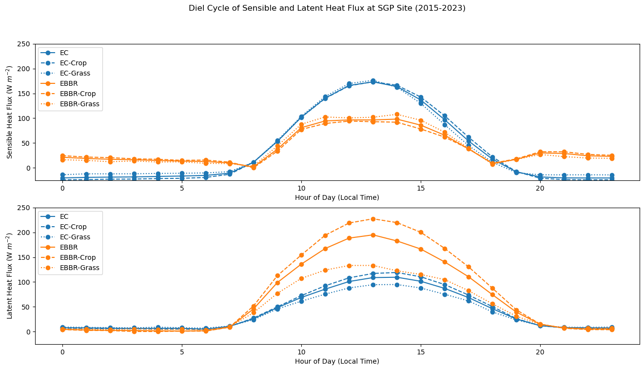

Footnotes¶

Location and Timeline of Flux Measurements at SGP from Sullivan et al. (2025)
↩
Gradients of temperature and humidity are measured above vegetation height using two sets of aspirated temperature and relative humidity (T /RH; Vaisala HMP45^[4]) probes mounted with a vertical separation of 1 m.
↩
Vaisala HMP45 Manual
↩
Net Radation is measured with Radiation and Energy Balance Systems (REBS), Inc, Q*7.1, REBS HFT-3 for soil heat flow, REBS STP-1 for soil temperature, and REBS SMP-2 for soil moisture.
↩

References¶

Sullivan, R. C., Billesbach, D. P., Biraud, S., Chan, S., Hart, R., Keeler, E., Kyrouac, J., Pal, S., Pekour, M., Sullivan, S. L., Theisen, A., Tuftedal, M., & Cook, D. R. (2025). Over three decades, and counting, of near-surface turbulent flux measurements from the Atmospheric Radiation Measurement (ARM) user facility. Earth System Science Data, 17(9), 5007–5038. 10.5194/essd-17-5007-2025
Sullivan, R., Billesbach, D., Keeler, E., Ermold, B., & Pal, S. (1997). Eddy Correlation Flux Measurement System (30ECOR), 2015-10-06 to 2019-10-23, Southern Great Plains (SGP), Morrison, OK (Extended) (E39). In Atmospheric Radiation Measurement (ARM) user facility. 10.5439/1025039
Sullivan, R., Cook, D., Shi, Y., Keeler, E., & Pal, S. (2019). Eddy Correlation Flux Measurement System (ECORSF), 2019-10-23 to 2026-03-12, Southern Great Plains (SGP), Morrison, OK (Extended) (E39). In Atmospheric Radiation Measurement (ARM) user facility. 10.5439/1494128
Sullivan, R., Ermold, B., Pal, S., & Keeler, E. (1993). Energy Balance Bowen Ratio Station (30EBBR), 2015-09-30 to 2023-12-17, Southern Great Plains (SGP), Morrison, OK (Extended) (E39). In Atmospheric Radiation Measurement (ARM) user facility. 10.5439/1023895