Plotting Data from a Field Campaign (TRACER)
Contents
Plotting Data from a Field Campaign (TRACER)#
Overview#
Within this notebook, we will cover:
How to access data from the Atmospheric Radiation Measurment (ARM) user facility
How to setup a workflow to plot both cross sections (RHIs) and horizontal scans (PPIs)
Prerequisites#
Concepts |
Importance |
Notes |
|---|---|---|
Required |
Basic plotting |
|
Py-ART Basics |
Required |
IO/Visualization |
Imports#
import glob
import os
from pathlib import Path

import act
import imageio.v2 as imageio
import matplotlib
import matplotlib.pyplot as plt
import pyart
## You are using the Python ARM Radar Toolkit (Py-ART), an open source
## library for working with weather radar data. Py-ART is partly
## supported by the U.S. Department of Energy as part of the Atmospheric
## Radiation Measurement (ARM) Climate Research Facility, an Office of
## Science user facility.
##
## If you use this software to prepare a publication, please cite:
##
##     JJ Helmus and SM Collis, JORS 2016, doi: 10.5334/jors.119
<frozen importlib._bootstrap>:283: DeprecationWarning: the load_module() method is deprecated and slated for removal in Python 3.12; use exec_module() instead
/Users/mgrover/miniforge3/envs/pyart-docs/lib/python3.10/site-packages/tqdm/auto.py:22: TqdmWarning: IProgress not found. Please update jupyter and ipywidgets. See https://ipywidgets.readthedocs.io/en/stable/user_install.html
  from .autonotebook import tqdm as notebook_tqdm
Grab Data from ARM#
One of the better cases was from June 2, 2022, where several cold pools and single-cell storms traversed through the domain.
The Tracking Aerosol Convection Interactions ExpeRiment (TRACER) Field Campaign#
Data is available from the Atmospheric Radiation Measurment user facility, which helped to lead the TRACER field campaign in Houston, Texas.
The data are available from the ARM data portal (https://adc.arm.gov/).
We are interested in the C-band radar, which is utilizing a cell-tracking algorithm, with the datastream
houcsapr2cfrS2.a1
Use the ARM Live API to Download the Data, using ACT#
The Atmospheric Data Community Toolkit (ACT) has a helpful module to interface with the data server:
act.discovery.download_data?
Signature:
act.discovery.download_data(
    username,
    token,
    datastream,
    startdate,
    enddate,
    time=None,
    output=None,
)
Docstring:
This tool will help users utilize the ARM Live Data Webservice to download
ARM data.

Parameters
----------
username : str
    The username to use for logging into the ADC archive.
token : str
    The access token for accessing the ADC archive.
datastream : str
    The name of the datastream to acquire.
startdate : str
    The start date of the data to acquire. Formats accepted are
    YYYY-MM-DD, DD.MM.YYYY, DD/MM/YYYY, YYYYMMDD, YYYY/MM/DD or
    any of the previous formats with THH:MM:SS added onto the end
    (ex. 2020-09-15T12:00:00).
enddate : str
    The end date of the data to acquire. Formats accepted are
    YYYY-MM-DD, DD.MM.YYYY, DD/MM/YYYY, YYYYMMDD or YYYY/MM/DD, or
    any of the previous formats with THH:MM:SS added onto the end
    (ex. 2020-09-15T13:00:00).
time: str or None
    The specific time. Format is HHMMSS. Set to None to download all files
    in the given date interval.
output : str
    The output directory for the data. Set to None to make a folder in the
    current working directory with the same name as *datastream* to place
    the files in.

Returns
-------
files : list
    Returns list of files retrieved

Notes
-----
This programmatic interface allows users to query and automate
machine-to-machine downloads of ARM data. This tool uses a REST URL and
specific parameters (saveData, query), user ID and access token, a
datastream name, a start date, and an end date, and data files matching
the criteria will be returned to the user and downloaded.

By using this web service, users can setup cron jobs and automatically
download data from /data/archive into their workspace. This will also
eliminate the manual step of following a link in an email to download data.
All other data files, which are not on the spinning
disk (on HPSS), will have to go through the regular ordering process.
More information about this REST API and tools can be found on `ARM Live
<https://adc.arm.gov/armlive/#scripts>`_.

To login/register for an access token click `here
<https://adc.arm.gov/armlive/livedata/home>`_.

Author: Michael Giansiracusa
Email: giansiracumt@ornl.gov

Web Tools Contact: Ranjeet Devarakonda zzr@ornl.gov

Examples
--------
This code will download the netCDF files from the sgpmetE13.b1 datastream
and place them in a directory named sgpmetE13.b1. The data from 14 Jan to
20 Jan 2017 will be downloaded. Replace *userName* and *XXXXXXXXXXXXXXXX*
with your username and token for ARM Data Discovery. See the Notes for
information on how to obtain a username and token.

.. code-block:: python

    act.discovery.download_data(
        "userName", "XXXXXXXXXXXXXXXX", "sgpmetE13.b1", "2017-01-14", "2017-01-20"
    )
File:      ~/miniforge3/envs/pyart-docs/lib/python3.10/site-packages/act/discovery/get_armfiles.py
Type:      function
Setup our Download Query#
Before downloading our data, we need to make sure we have an ARM Data Account, and ARM Live token. Both of these can be found using this link:
Once you sign up, you will see your token. Copy and replace that where we have arm_username and arm_password below.
arm_username = os.getenv("ARM_USERNAME")
arm_password = os.getenv("ARM_PASSWORD")

datastream = "houcsapr2cfrS2.a1"

start_date = "2022-06-17T19:00:00"
end_date = "2022-06-17T19:05:00"

print(len(arm_username), len(arm_password))
8 16
csapr_files = act.discovery.download_data(arm_username,
                                          arm_password,
                                          datastream,
                                          start_date,
                                          end_date)
[DOWNLOADING] houcsapr2cfrS2.a1.20220617.190219.nc
[DOWNLOADING] houcsapr2cfrS2.a1.20220617.190312.nc
[DOWNLOADING] houcsapr2cfrS2.a1.20220617.190448.nc
[DOWNLOADING] houcsapr2cfrS2.a1.20220617.190237.nc
[DOWNLOADING] houcsapr2cfrS2.a1.20220617.190154.nc
[DOWNLOADING] houcsapr2cfrS2.a1.20220617.190027.nc
[DOWNLOADING] houcsapr2cfrS2.a1.20220617.190001.nc
[DOWNLOADING] houcsapr2cfrS2.a1.20220617.190057.nc
[DOWNLOADING] houcsapr2cfrS2.a1.20220617.190145.nc
[DOWNLOADING] houcsapr2cfrS2.a1.20220617.190106.nc
[DOWNLOADING] houcsapr2cfrS2.a1.20220617.190325.nc
[DOWNLOADING] houcsapr2cfrS2.a1.20220617.190246.nc
[DOWNLOADING] houcsapr2cfrS2.a1.20220617.190358.nc
[DOWNLOADING] houcsapr2cfrS2.a1.20220617.190414.nc
[DOWNLOADING] houcsapr2cfrS2.a1.20220617.190041.nc
[DOWNLOADING] houcsapr2cfrS2.a1.20220617.190132.nc
[DOWNLOADING] houcsapr2cfrS2.a1.20220617.190334.nc
[DOWNLOADING] houcsapr2cfrS2.a1.20220617.190424.nc
csapr_files = sorted(glob.glob('houcsapr2cfrS2.a1/houcsapr2cfrS2.a1.20220617.19*'))
Read in and Plot the Data#
Before following running the next cells, make sure you have created the following directories:
quicklooks/ppiquicklooks/rhiquicklooks/vpt
!mkdir quicklooks
!mkdir quicklooks/rhi
!mkdir quicklooks/ppi
!mkdir quicklooks/vpt
mkdir: quicklooks: File exists
mkdir: quicklooks/rhi: File exists
mkdir: quicklooks/ppi: File exists
mkdir: quicklooks/vpt: File exists
Loop through and plot#
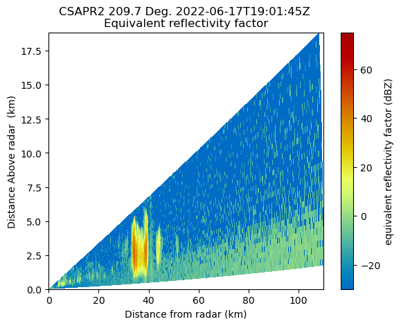
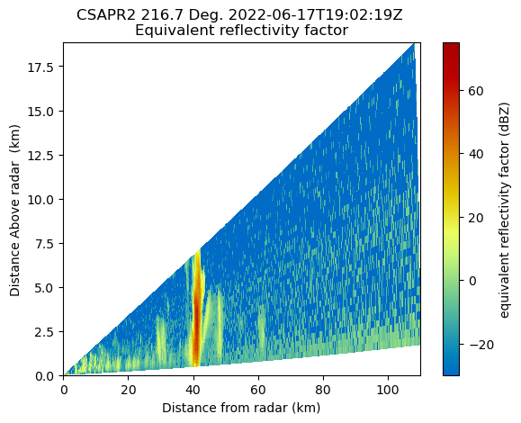
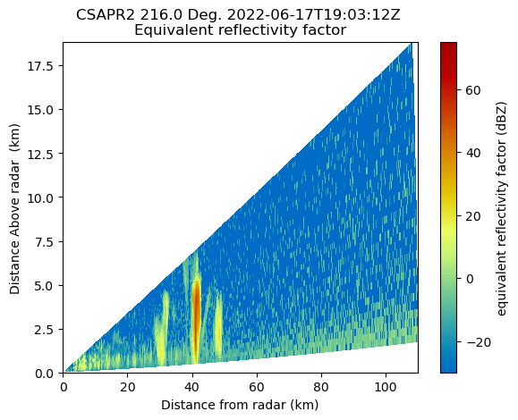
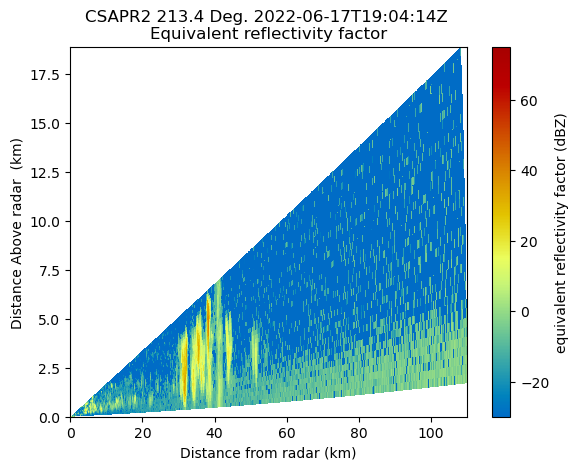
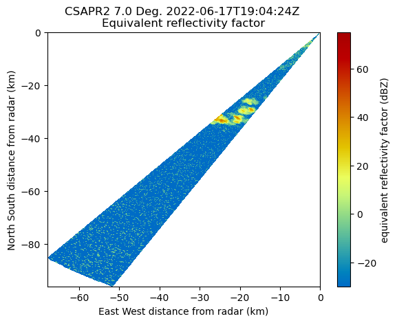
We read in the data, check the scan type, and plot a basic RadarDisplay which will automatically detect whether the plot is a vertical cross section (RHI or VPT), or a horizontal scan (PPI).
This offers a solid “quick look”, or initial visualization of the data.
for file in csapr_files:
    radar = pyart.io.read(file)
    print(radar.scan_type)
    display = pyart.graph.RadarDisplay(radar)
    display.plot("reflectivity", 0)
    plt.savefig(f"quicklooks/{radar.scan_type}/{Path(file).stem}.png", dpi=200)
    plt.show()
    plt.close()
ppi

rhi

rhi

rhi

ppi

rhi

rhi
ppi

rhi
rhi

ppi

rhi
rhi

ppi

rhi

rhi
ppi
rhi

Refine our Plot, Plot Velocity#
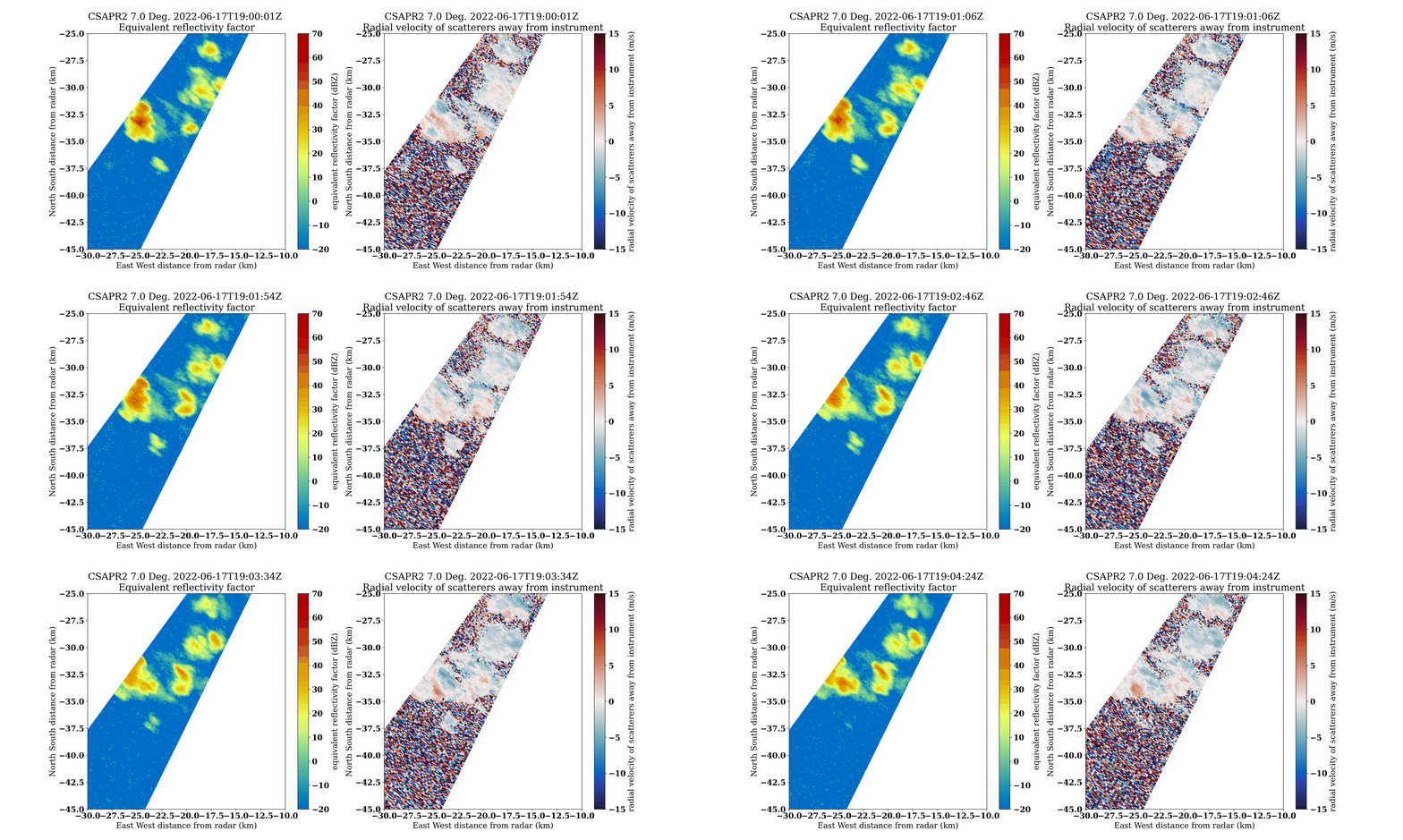
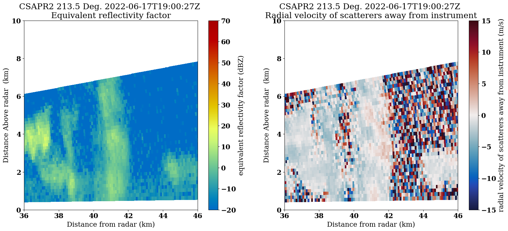
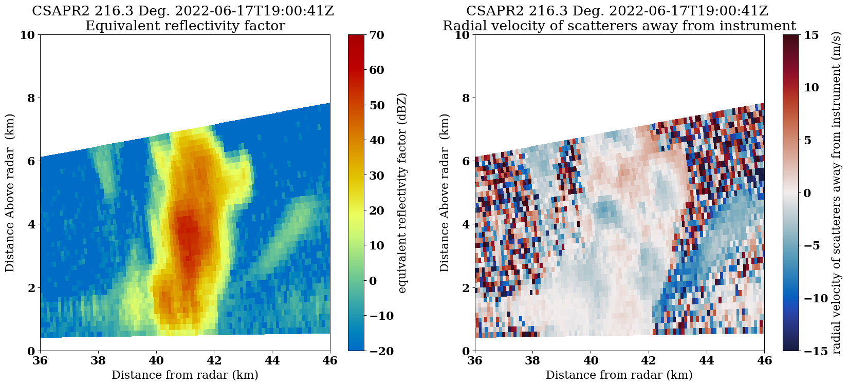
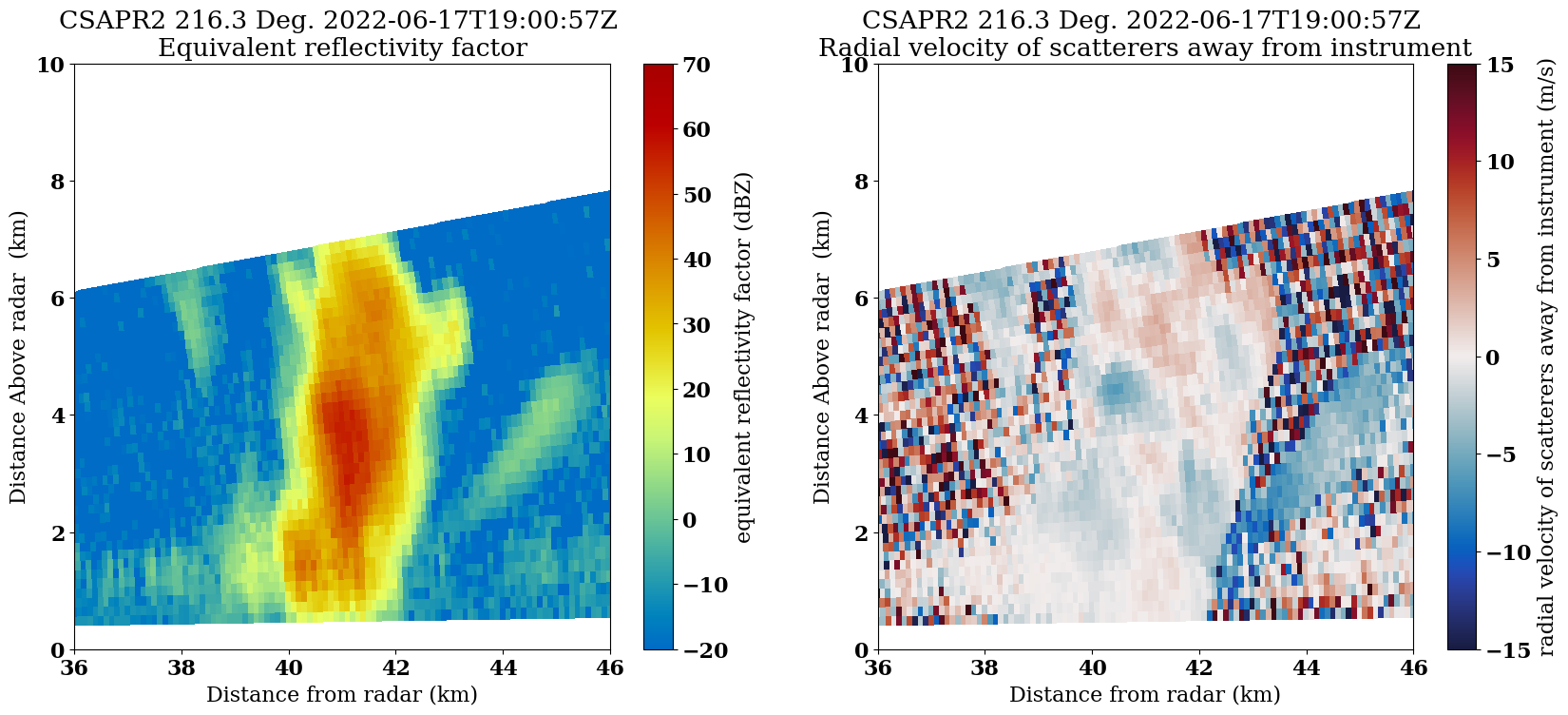
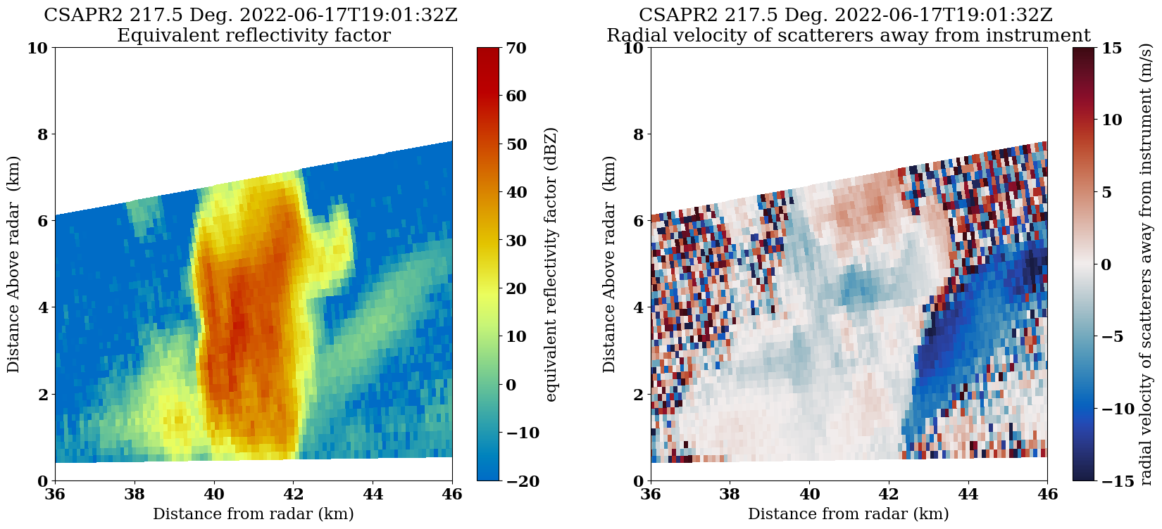
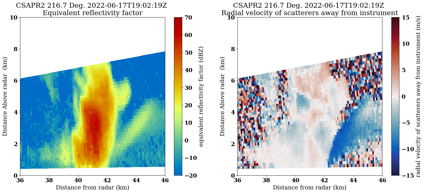
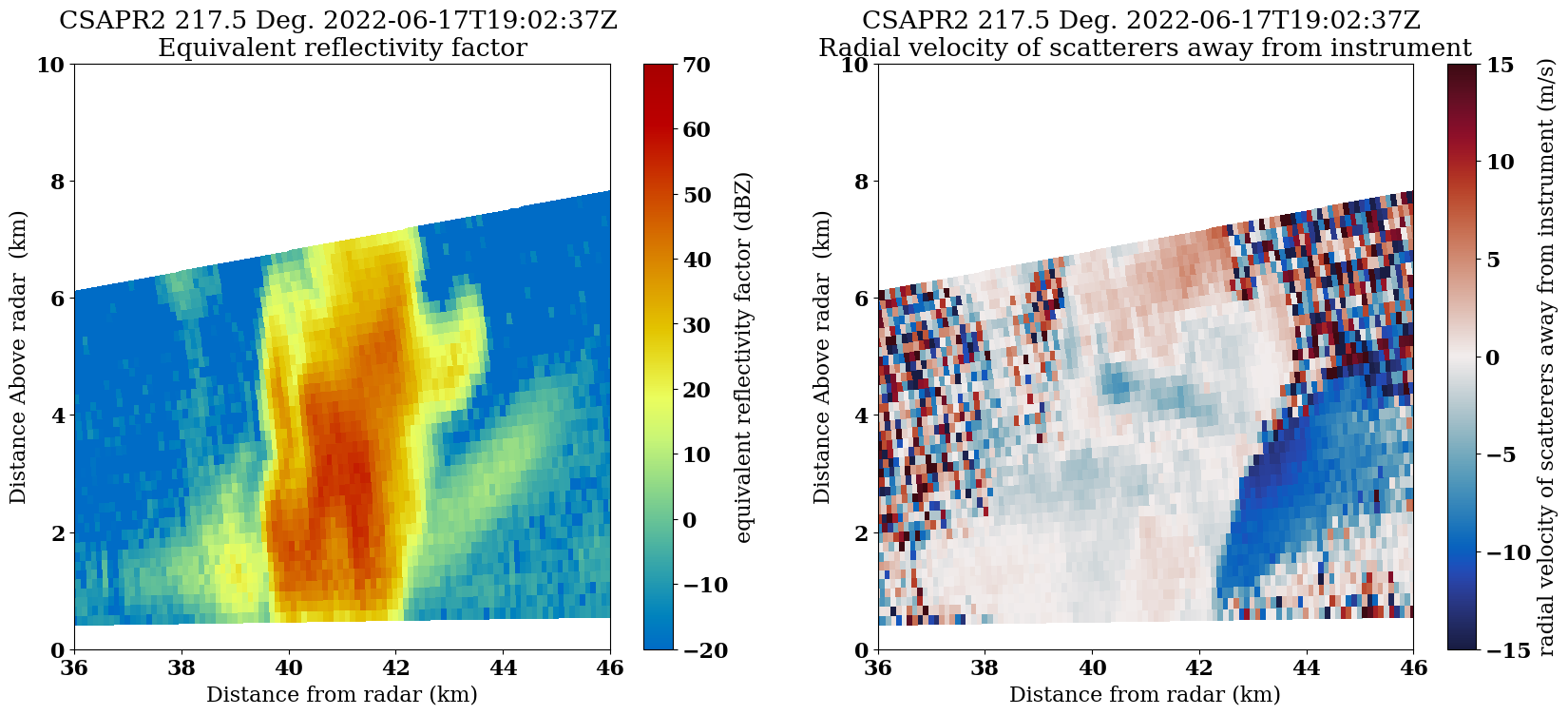
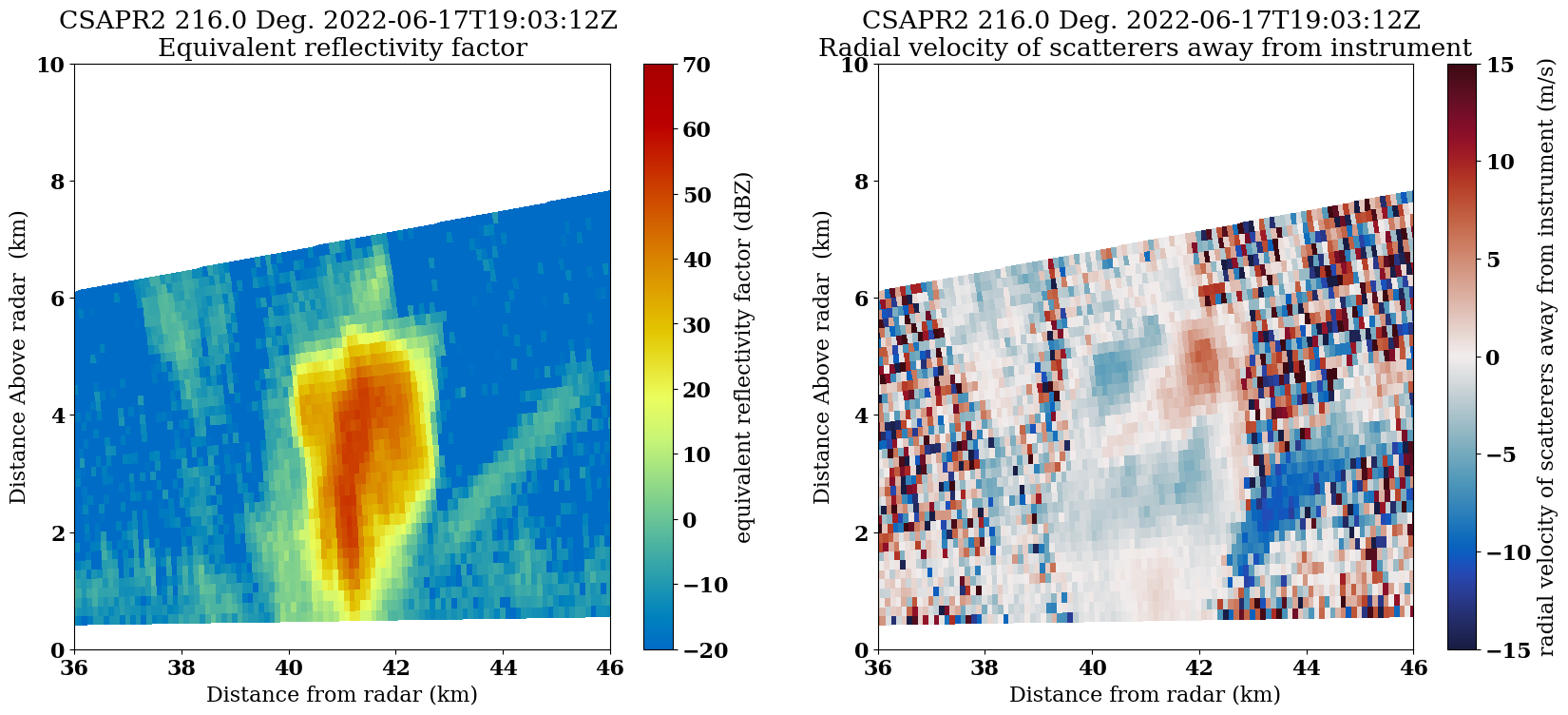
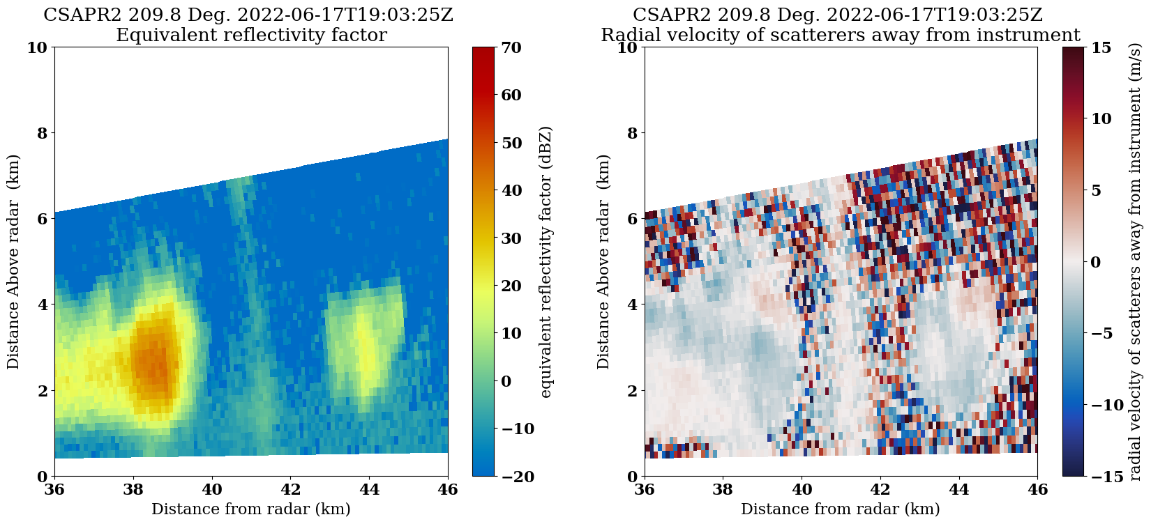
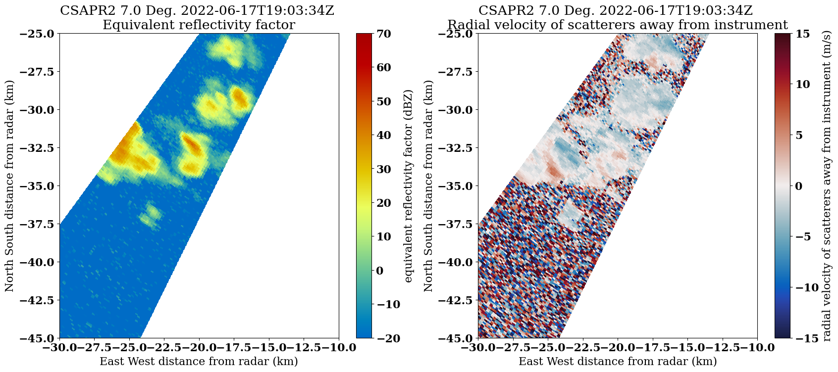
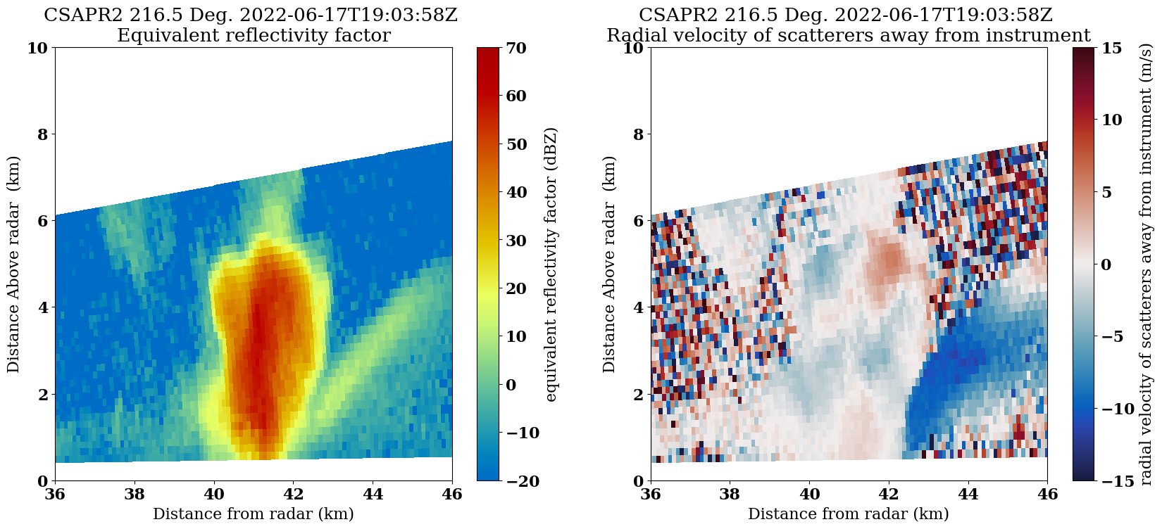
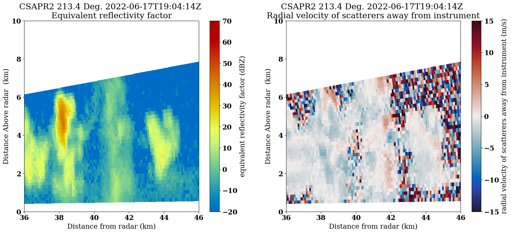
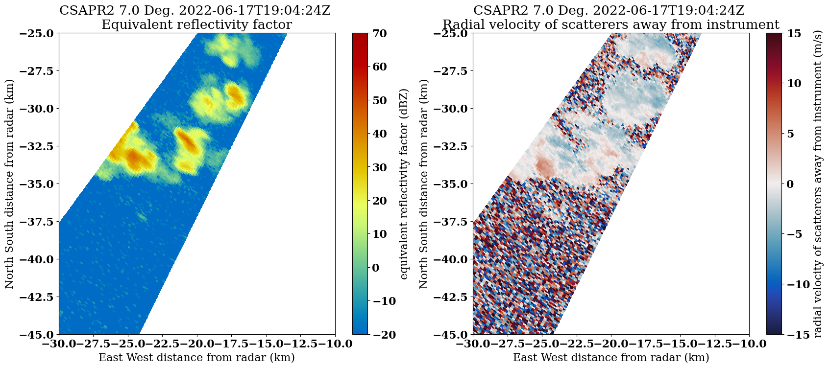
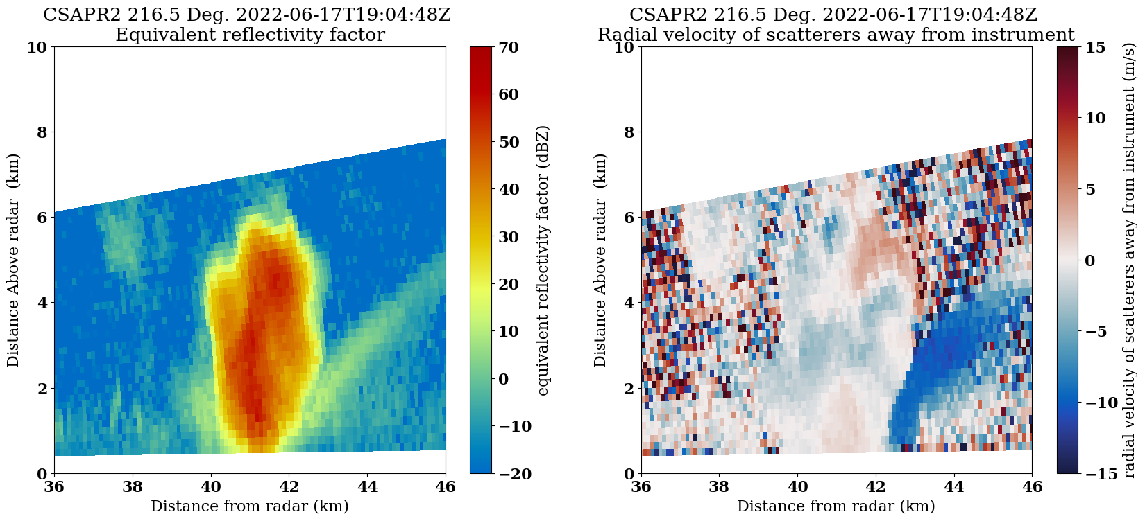
Let’s focus on the vertical scans of the data, or the RHIs.
You’ll notice that we had some cells around 60 km from the radar, with the vertical axis less than 6 km.
Let’s reflect that in the plots!
Customize our plot look#
Before we plot, we can change the size of our font, and style using the following parameters:
font = {'family' : 'serif',
        'weight' : 'bold',
        'size'   : 16}

matplotlib.rc('font', **font)

xlim_dict = {'ppi':(-30, -10),
             'rhi':(36, 46)
            }

ylim_dict = {'ppi':(-45, -25),
             'rhi':(0, 10)
            }
Apply our Plotting Loop#
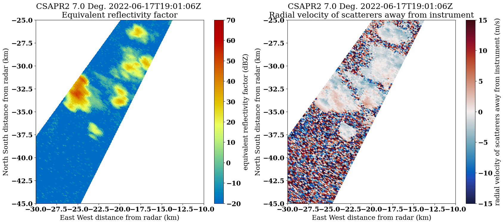
We:
Check to see if the scan is an RHI
Plot the reflectivity on one subplot
Plot velocity on the other
Save our plots
for file in csapr_files:
    radar = pyart.io.read(file)
    if (radar.scan_type == 'rhi' or radar.scan_type == 'ppi'):
        xlim = xlim_dict[radar.scan_type]
        ylim = ylim_dict[radar.scan_type]

        fig = plt.figure(figsize=(20,8))
        display = pyart.graph.RadarDisplay(radar)
        ax = plt.subplot(121)
        display.plot("reflectivity",
                     0,
                     ax=ax,
                     vmin=-20,
                     vmax=70)
        plt.xlim(xlim)
        plt.ylim(ylim)

        ax2 = plt.subplot(122)
        display.plot("mean_doppler_velocity",
                     0,
                     ax=ax2,
                     cmap='pyart_balance',
                     vmin=-15,
                     vmax=15)
        plt.xlim(xlim)
        plt.ylim(ylim)
        plt.savefig(f"quicklooks/{radar.scan_type}/{Path(file).stem}.png", dpi=200)
        plt.show()
        plt.close()




Create a GIF of teh RHI images#
rhi_images = sorted(glob.glob("quicklooks/rhi/*"))
ppi_images = sorted(glob.glob('quicklooks/ppi/*'))
with imageio.get_writer('rhi-animation.gif', mode='I') as writer:
    for filename in rhi_images:
        image = imageio.imread(filename)
        writer.append_data(image)

with imageio.get_writer('ppi-animation.gif', mode='I') as writer:
    for filename in ppi_images:
        image = imageio.imread(filename)
        writer.append_data(image)
Summary#
Within this example, we walked through how to access ARM data from a field campaign in Texas, plot a quick look of the data, and refine our plots to investigate a storm!
What’s Next?#
We will showcase other data workflow examples, including field campaigns in other regions and data access methods from other data centers.
Resources and References#
CSAPR Radar Data:
Bharadwaj, N., Collis, S., Hardin, J., Isom, B., Lindenmaier, I., Matthews, A., & Nelson, D. C-Band Scanning ARM Precipitation Radar (CSAPR2CFR). Atmospheric Radiation Measurement (ARM) User Facility. https://doi.org/10.5439/1467901
Py-ART:
Helmus, J.J. & Collis, S.M., (2016). The Python ARM Radar Toolkit (Py-ART), a Library for Working with Weather Radar Data in the Python Programming Language. Journal of Open Research Software. 4(1), p.e25. DOI: http://doi.org/10.5334/jors.119
ACT:
Adam Theisen, Ken Kehoe, Zach Sherman, Bobby Jackson, Alyssa Sockol, Corey Godine, Max Grover, Jason Hemedinger, Jenni Kyrouac, Maxwell Levin, Michael Giansiracusa (2022). The Atmospheric Data Community Toolkit (ACT). Zenodo. DOI: https://doi.org/10.5281/zenodo.6712343


