Bankhead National Forest - SACR RHI Investigation
Overview
As a part of standard quality control procedures for ARM radars, one system is typically matched to another for cross-comparison of specific parameters (e.g. reflectivity, differential reflectivity, etc).
As a standard procedure for the Ka-band Scanning Arm Cloud Radar (Ka-SACR), columns from the range height indictator (RHI) scans over the Ka-band Zenith Radar (KAZR) are extracted for comparison.
Investigation into the column extraction from a RHI scan has been requested.
Prerequisites
| Concepts | Importance | Notes |
|---|---|---|
| Intro to Cartopy | Necessary | |
| Understanding of NetCDF | Helpful | Familiarity with metadata structure |
| GeoPandas | Necessary | Familiarity with Geospatial Plotting |
| Py-ART / Radar Foundations | Necessary | Basics of Weather Radar |
Time to learn: 30 minutes
BNF Site Locations
| Site | Lat | Lon |
|---|---|---|
| M1 | 34.34525 | -87.33842 |
| S4 | 34.46451 | -87.23598 |
| S20 | 34.65401 | -87.29264 |
| S30 | 34.38501 | -86.92757 |
| S40 | 34.17932 | -87.45349 |
| S10. | 34.34361 | -87.35027 |
| S13. | 34.34388 | -87.35055 |
| S14. | 34.34333 | -87.35083 |
import warnings
warnings.filterwarnings("ignore", category=DeprecationWarning)

import glob
import os
import datetime
import tempfile
from datetime import timedelta

import numpy as np
import matplotlib.pyplot as plt
import matplotlib.gridspec as gridspec
import xarray as xr
import pandas as pd
import dask
import cartopy
import cartopy.crs as ccrs

from math import atan2 as atan2
from cartopy import crs as ccrs, feature as cfeature
from cartopy.io.img_tiles import OSM
from matplotlib.transforms import offset_copy
from mpl_toolkits.axes_grid1 import make_axes_locatable
from mpl_toolkits.axisartist.grid_finder import FixedLocator, DictFormatter
from matplotlib import colors
from dask.distributed import Client, LocalCluster
from metpy.plots import USCOUNTIES
from PIL import Image
from scipy.signal import find_peaks

import act
import pyart
import wradlib as wrl
import cmweather
import xradar as xd

dask.config.set({'logging.distributed': 'error'})
## You are using the Python ARM Radar Toolkit (Py-ART), an open source
## library for working with weather radar data. Py-ART is partly
## supported by the U.S. Department of Energy as part of the Atmospheric
## Radiation Measurement (ARM) Climate Research Facility, an Office of
## Science user facility.
##
## If you use this software to prepare a publication, please cite:
##
##     JJ Helmus and SM Collis, JORS 2016, doi: 10.5334/jors.119
<dask.config.set at 0x7feb32e37490>Define Functions
def subset_points(nfile, **kwargs):
    """
    Subset a radar file for a set of latitudes and longitudes
    utilizing Py-ART's get_field_location functionality.

    Parameters
    ----------
    file : str
        Path to the radar file to extract columns from
    nsonde : list
        List containing file paths to the desired sonde file to merge

    Calls
    -----
    radar_start_time
    merge_sonde

    Returns
    -------
    ds : xarray DataSet
        Xarray Dataset containing the radar column above a give set of locations

    """
    ds = None

    # Define the splash locations [lon,lat]
    M1 = [34.34525, -87.33842]
    S13 = [34.343889, -87.350556]

    sites    = ["M1", "S13"]
    site_alt = [293, 286]

    # Zip these together!
    lats, lons = list(zip(M1,
                          S13))
    try:
        # Read in the file
        radar = pyart.io.read(nfile)
        # Check for single sweep scans
        if np.ma.is_masked(radar.sweep_start_ray_index["data"][1:]):
            radar.sweep_start_ray_index["data"] = np.ma.array([0])
            radar.sweep_end_ray_index["data"] = np.ma.array([radar.nrays])
    except:
        radar = None

    if radar:
        if radar.scan_type != "rhi":
            if radar.time['data'].size > 0:

                column_list = []
                for lat, lon in zip(lats, lons):
                    # Make sure we are interpolating from the radar's location above sea level
                    # NOTE: interpolating throughout Troposphere to match sonde to in the future
                    try:
                        da = (
                            pyart.util.columnsect.get_field_location(radar, lat, lon)
                            .interp(height=np.arange(500, 8500, 200))
                        )
                    except ValueError:
                        da = pyart.util.columnsect.get_field_location(radar, lat, lon)
                        # check for valid heights
                        valid = np.isfinite(da["height"])
                        n_valid = int(valid.sum())
                        if n_valid > 0:
                            da = da.sel(height=valid).sortby("height").interp(height=np.arange(500, 8500, 200))
                        else:
                            target_height = xr.DataArray(np.arange(500, 8500, 200), dims="height", name="height")
                            da = da.reindex(height=target_height)

                    # Add the latitude and longitude of the extracted column
                    da["lat"], da["lon"] = lat, lon
                    # Convert timeoffsets to timedelta object and precision on datetime64
                    ##da.time_offset.data = da.time_offset.values.astype("timedelta64[s]")
                    da.base_time.data = da.base_time.values.astype("datetime64[s]")
                    column_list.append(da)

                # Concatenate the extracted radar columns for this scan across all sites
                ds = xr.concat([data for data in column_list if data], dim='station')
                ds["station"] = sites
                # Assign the Main and Supplemental Site altitudes
                ds = ds.assign(alt=("station", site_alt))
                ds.station.attrs.update(long_name="Bankhead National Forest AMF-3 In-Situ Ground Observation Station Identifers")
                ds.lat.attrs.update(long_name='Latitude of BNF AMF-3 Ground Observation Site',
                                         units='Degrees North')
                ds.lon.attrs.update(long_name='Longitude of BNF AMF-3 Ground Observation Site',
                                          units='Degrees East')
                ds.alt.attrs.update(long_name="Altitude above mean sea level for each station",
                                          units="m")
                # delete the radar to free up memory
                del radar, column_list, da
            else:
                # delete the rhi file
                del radar
        else:
            del radar
    return ds
def gc_latlon_bear_dist(lat1, lon1, bear, dist):
"""
Input lat1/lon1 as decimal degrees, as well as bearing and distance from
the coordinate. Returns lat2/lon2 of final destination. Cannot be
vectorized due to atan2.
"""
re = 6371.1 # km
lat1r = np.deg2rad(lat1)
lon1r = np.deg2rad(lon1)
bearr = np.deg2rad(bear)
lat2r = np.arcsin((np.sin(lat1r) * np.cos(dist/re)) +
(np.cos(lat1r) * np.sin(dist/re) * np.cos(bearr)))
lon2r = lon1r + atan2(np.sin(bearr) * np.sin(dist/re) *
np.cos(lat1r), np.cos(dist/re) - np.sin(lat1r) *
np.sin(lat2r))
return np.rad2deg(lat2r), np.rad2deg(lon2r)
def add_scale_line(scale, ax, projection, color='k',
linewidth=None, fontsize=None, fontweight=None):
"""
Adds a line that shows the map scale in km. The line will automatically
scale based on zoom level of the map. Works with cartopy.
Parameters
----------
scale : scalar
Length of line to draw, in km.
ax : matplotlib.pyplot.Axes instance
Axes instance to draw line on. It is assumed that this was created
with a map projection.
projection : cartopy.crs projection
Cartopy projection being used in the plot.
Other Parameters
----------------
color : str
Color of line and text to draw. Default is black.
"""
frac_lat = 0.1 # distance fraction from bottom of plot
frac_lon = 0.5 # distance fraction from left of plot
e1 = ax.get_extent()
center_lon = e1[0] + frac_lon * (e1[1] - e1[0])
center_lat = e1[2] + frac_lat * (e1[3] - e1[2])
# Main line
lat1, lon1 = gc_latlon_bear_dist(
center_lat, center_lon, -90, scale / 2.0) # left point
lat2, lon2 = gc_latlon_bear_dist(
center_lat, center_lon, 90, scale / 2.0) # right point
if lon1 <= e1[0] or lon2 >= e1[1]:
warnings.warn('Scale line longer than extent of plot! ' +
'Try shortening for best effect.')
ax.plot([lon1, lon2], [lat1, lat2], linestyle='-',
color=color, transform=projection,
linewidth=linewidth)
# Draw a vertical hash on the left edge
lat1a, lon1a = gc_latlon_bear_dist(
lat1, lon1, 180, frac_lon * scale / 20.0) # bottom left hash
lat1b, lon1b = gc_latlon_bear_dist(
lat1, lon1, 0, frac_lon * scale / 20.0) # top left hash
ax.plot([lon1a, lon1b], [lat1a, lat1b], linestyle='-',
color=color, transform=projection, linewidth=linewidth)
# Draw a vertical hash on the right edge
lat2a, lon2a = gc_latlon_bear_dist(
lat2, lon2, 180, frac_lon * scale / 20.0) # bottom right hash
lat2b, lon2b = gc_latlon_bear_dist(
lat2, lon2, 0, frac_lon * scale / 20.0) # top right hash
ax.plot([lon2a, lon2b], [lat2a, lat2b], linestyle='-',
color=color, transform=projection, linewidth=linewidth)
# Draw scale label
ax.text(center_lon, center_lat - frac_lat * (e1[3] - e1[2]) / 3.0,
str(int(scale)) + ' km', horizontalalignment='center',
verticalalignment='center', color=color, fontweight=fontweight,
fontsize=fontsize)def bnf_display(radar,
field="reflectivity",
vmin=-40,
vmax=5):
"""
Create a display to visualize radar reflectivity across
the domain, marking locations of the BNF sites.
Input
-----
radar : str
Path to radar file
field : str
Specific radar parameter to display
vmin : int
Minimum value to display between all subplots for the specific radar
parameter
vmax : int
Maximum value to display between all subplots for the specific radar
parameter
Returns
-------
fig : matplotlib figure
returns a figure object for display
"""
#------------------
# Inputs
#------------------
# Open the files
try:
radar = pyart.io.read(radar)
# skip the RHI scans for now
if radar.scan_type != "ppi":
print("rhi file")
return
# check for those weird files
if radar.elevation['data'].shape[0] < 1:
return
except:
return
# define the sites of interest
nsite = {"M1" : [34.34525, -87.33842],
"S4" : [34.46451, -87.23598],
"S3" : [34.63080, -87.13311],
"S20" : [34.65401, -87.29264]}
# define the center of the map to be the CSAPR2
central_lon = -87.13076
central_lat = 34.63080
#-------------------
# Define the Figure
#-------------------
fig = plt.figure(figsize=(16, 8))
tiler = OSM()
mercator = tiler.crs
#--------------------------------------
# Main Plot - Display the CMAC Field
#--------------------------------------
# Create a subplot and define projection
ax = fig.add_subplot(111, projection=ccrs.PlateCarree())
# Add some various map elements to the plot to make it recognizable.
ax.add_feature(cfeature.COASTLINE)
ax.add_image(tiler, 9, zorder=2, alpha=0.35)
# Set the BNF Domain (adjust later for various groups)
ax.set_extent([272.5, 273.0, 34.7, 34.2])
gl = ax.gridlines(draw_labels=True)
# Hide the right side ticks
ax.tick_params(labeltop=False, labelright=False)
# Add the column sites
markers = ["p", "*", "+", "D", "o", "s"]
for i, site in enumerate(nsite):
ax.scatter(nsite[site][1],
nsite[site][0],
marker=markers[i],
color="black",
s=75,
label=site,
zorder=3,
transform=ccrs.PlateCarree())
# Use the cartopy interface to create a matplotlib transform object
# for the Geodetic coordinate system. We will use this along with
# matplotlib's offset_copy function to define a coordinate system which
# translates the text by 25 pixels to the left.
# note - taken from cartopy examples
geodetic_transform = ccrs.PlateCarree()._as_mpl_transform(ax)
text_transform = offset_copy(geodetic_transform, units='dots', x=+50, y=+15)
if site == "S3":
# Add text 25 pixels to the left of the volcano.
ax.text(nsite[site][1]-0.01,
nsite[site][0],
"CSAPR-2",
verticalalignment='center',
horizontalalignment='right',
transform=text_transform,
bbox=dict(facecolor='sandybrown',
alpha=0.5,
boxstyle='round'))
else:
# Add text 25 pixels to the left of the volcano.
ax.text(nsite[site][1]-0.01,
nsite[site][0],
site,
verticalalignment='center',
horizontalalignment='right',
transform=text_transform,
bbox=dict(facecolor='sandybrown',
alpha=0.5,
boxstyle='round'))
display = pyart.graph.RadarMapDisplay(radar)
display.plot_ppi_map(field,
vmin=vmin,
vmax=vmax,
ax=ax,
cmap="ChaseSpectral",
zorder=1,
colorbar_flag=False,
)
ims = display.plots[0]
cbar = fig.colorbar(ims, ax=ax, location="bottom", shrink=0.6, pad=0.1)
cbar_label = (radar.fields["reflectivity"]["long_name"] +
'\n [' +
radar.fields["reflectivity"]["units"] + ']'
)
cbar.set_label(cbar_label)
# Add our scale bar
add_scale_line(20.0, ax, projection=ccrs.PlateCarree(),
color='black', linewidth=3,
fontsize=12,
fontweight='bold')
return fig
Read the Ka-SACR Data with xradar
# Define the desired processing date for the BNF CSAPR-2 in YYYY-MM-DD format.
DATE = "20250425"
# Define the directory where the BNF CSAPR-2 CMAC files are located.
RADAR_DIR = sorted(glob.glob(os.getenv("BNF_SACR_DIR") + "*." + DATE + ".*.nc"))
Initial Look at the Data
dt = xd.io.open_cfradial1_datatree(RADAR_DIR[1])dtLoading...
dt['sweep_2']['reflectivity'].plot(vmax=0)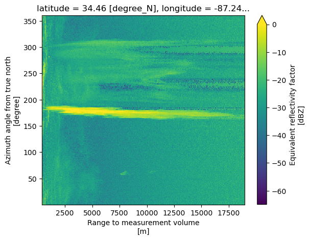
fig = plt.figure(figsize=[10, 10])
radar = pyart.xradar.Xradar(dt)
display = pyart.graph.RadarDisplay(radar)
display.plot_ppi("reflectivity", vmax=5)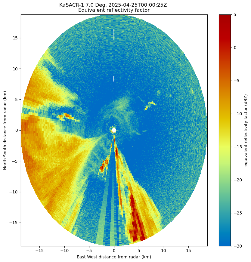
Convert from xradar to BNF Display
outfig = bnf_display(RADAR_DIR[1])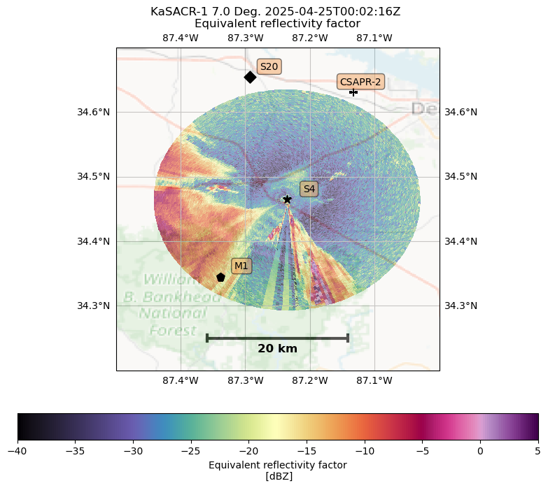
Column Extraction
Single Column - PPI
single_column = pyart.util.columnsect.get_field_location(radar, 34.34525, -87.33842)single_columnLoading...
single_column.reflectivity.plot(y='height')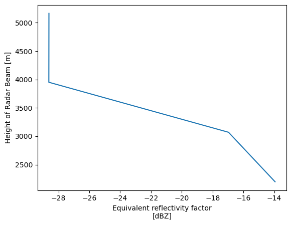
All PPI Scans
%%time
## Start up a Dask Cluster
columns = []
for file in RADAR_DIR:
    columns.append(subset_points(file))
CPU times: user 1min 3s, sys: 3.07 s, total: 1min 6s
Wall time: 1min 7s
# Concatenate all extracted columns across time dimension to form daily timeseries
ppi = xr.concat([data for data in columns if data], dim="time")
# Drop unnecessary time dimensions from a few required ARM spatial variables
ppi['time'] = ppi.sel(station="M1").base_time
ppi['time_offset'] = ppi.sel(station="M1").base_time
ppi['base_time'] = ppi.sel(station="M1").isel(time=0).base_time
ppi['lat'] = ppi.isel(time=0).lat
ppi['lon'] = ppi.isel(time=0).lon
ppi['alt'] = ppi.isel(time=0).altppiLoading...
ppi.sel(station="M1").sel(time=slice("2025-04-25T03:00:00", "2025-04-25T06:00:00")).reflectivity.plot(x='time')
Single Column - RHI
radar_rhi = pyart.io.read(RADAR_DIR[2])
radar_rhi.scan_type'rhi'display = pyart.graph.RadarDisplay(radar_rhi)display.plot("reflectivity", vmax=5)
rhi_column = pyart.util.columnsect.get_field_location(radar_rhi, 34.34525, -87.33842)rhi_columnLoading...
rhi_column.reflectivity.plot(y='height')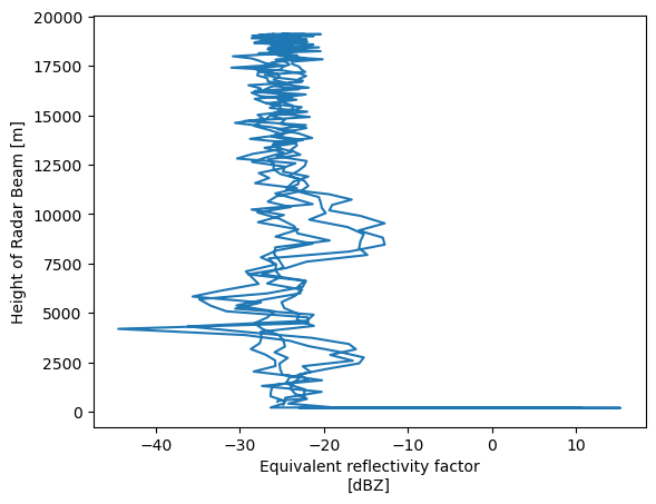
rhi_column.time_offset.plot(y="height")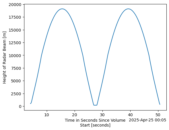
def split_column(column, height_range=[500, 8500], height_interp=200):
    """
    For Extracted Columns from RHI scans, height values are not unique,
    limiting the ability to interpolate across the entire date to
    standardize gates

    Given a column, find the peaks within the distribution, and split the
    column into separate instances with unique height values

    Inputs
    ------
    column : xarray DataSet
        extracted column for a specific site
    height_range : list [min, max]
        Height Range to interpolate each column split
    height_interp : int
        Frequency between height gates used within interpolation

    Outputs
    -------
    split_column : list
        From the peaks (p) within the height distribution, peaks are split into
        separate columns and returned to the user as a list of xarray DataSets.

    """

    # Determine the peaks within extracted column
    peaks, _ = find_peaks(column['height'], prominence=1)

    if len(peaks) > 1:
        # Before first peak
        column_a = column.isel(height=slice(0, peaks[0])).interp(
            height=np.arange(height_range[0], height_range[1], height_interp))
        column_a['base_time'] = column.isel(height=slice(0, peaks[0])).time_offset.data[-1]
        # First Peak to Minimium
        column_b = column.isel(height=slice(peaks[0], int(column.height.argmin()))).interp(
            height=np.arange(height_range[0], height_range[1], height_interp))
        column_b['base_time'] = column.isel(height=slice(peaks[0], int(column.height.argmin()))).time_offset.data[-1]
        # Minimum to 2nd Peak
        column_c = column.isel(height=slice(int(column.height.argmin()+1), peaks[1])).interp(
            height=np.arange(height_range[0], height_range[1], height_interp))
        column_c['base_time'] = column.isel(height=slice(int(column.height.argmin()+1), peaks[1])).time_offset.data[-1]
        # 2nd Peak to end
        column_d = column.isel(height=slice(peaks[1], len(column.height))).interp(
            height=np.arange(height_range[0], height_range[1], height_interp))
        column_d['base_time'] = column.isel(height=slice(peaks[1], len(column.height))).time_offset.data[-1]
        split_column = [column_a, column_b, column_c, column_d]
    else:
        column_a = column.isel(height=slice(0, peaks[0])).interp(
            height=np.arange(height_range[0], height_range[1], height_interp))
        column_b = column.isel(height=slice(peaks[0], int(rhi_column.height.argmin()))).interp(
            height=np.arange(height_range[0], height_range[1], height_interp))
        split_column = [column_a, column_b]

    return split_column
out_column = split_column(rhi_column)out_column[2]Loading...
rhi_single = xr.concat([data for data in out_column if data], dim="time")
rhi_single['time'] = rhi_single['base_time']
rhi_single.reflectivity.plot(x='time')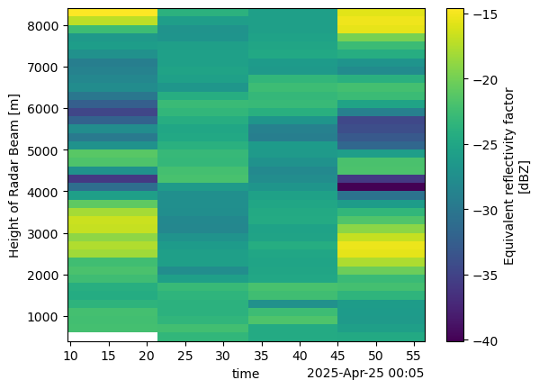
All RHI Columns
merge_columns = []

for file in RADAR_DIR:
    radar = pyart.io.read(file)
    if radar.scan_type == "rhi":
        rhi_column = pyart.util.columnsect.get_field_location(radar, 34.34525, -87.33842)
        out_column = split_column(rhi_column)
        merge_columns.extend(out_column)

        del radar
rhi = xr.concat([data for data in merge_columns if data], dim="time")
# Drop unnecessary time dimensions from a few required ARM spatial variables
rhi['time'] = rhi.base_timerhi.reflectivity.sel(time=slice("2025-04-25T03:00:00", "2025-04-25T06:00:00")).plot(y='height')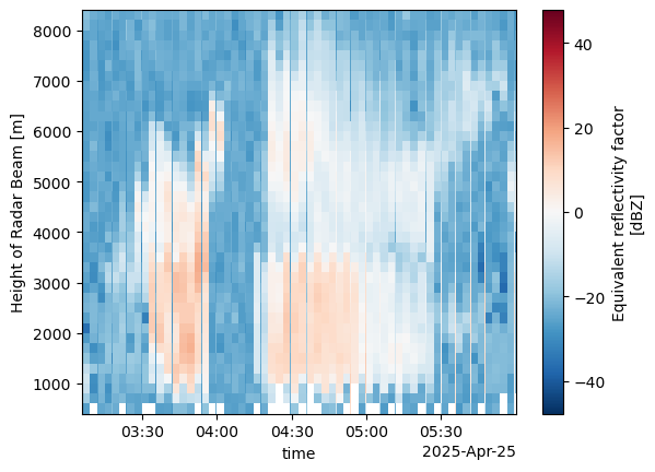
rhi = rhi.assign_coords(station="M1")
rhi
Loading...
Merged PPI + RHI Column Extraction
ppi = ppi.drop_vars({"base_time", "time_offset"})rhi = rhi.drop_vars({"base_time"})datasets = [ds_val for ds_val in [rhi, ppi] if isinstance(ds_val, xr.Dataset)]combined_column = xr.merge(datasets)combined_columnLoading...
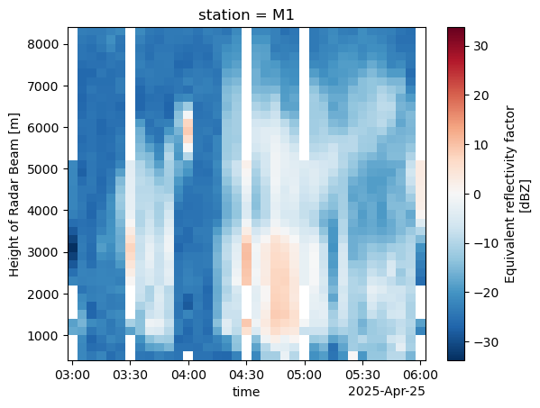
combined_column.sel(station="M1").sel(time=slice("2025-04-25T03:00:00", "2025-04-25T06:00:00")).reflectivity.plot(x='time')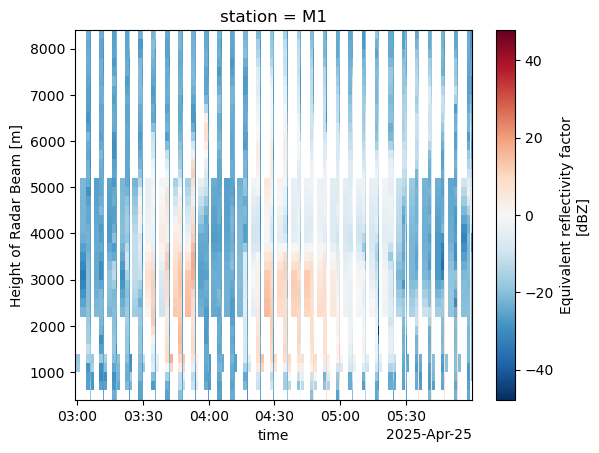
combined_column.resample(time="5Min").mean().sel(station="M1").sel(time=slice("2025-04-25T03:00:00", "2025-04-25T06:00:00")).reflectivity.plot(x='time')